Quickstart

In this brief tutorial, we’ll run a quick simulation that illustrates the impact of cross-trait assortative mating on the the Haseman-Elston regression genetic correlation estimator. In the process, we’ll learning about the essential components of an xftsim simulation.

Setting up a simulation

import xftsim as xft
from xftsim.sim import Simulation
import numpy as np
import pandas as pd
import seaborn as sns

xft.config.print_durations_threshold=10. ## reduce verbosity
np.random.seed(123) ## set random seed for reproducibility

Simulation objects require the following arguments:

• founder_haplotypes: xarray.core.dataarray.DataArray,

• architecture: xftsim.arch.Architecture,

• recombination_map: xftsim.reproduce.RecombinationMap,

• mating_regime: xftsim.mate.MatingRegime,

Together, these comprise our initial generation’s haplotypes (founder_haplotypes), a phenogenetic architecture mapping genotypes to phenotypes (architecture), a method for assigning mates (mating_regime), and a recombination map for meiosis (recombination_map).

We can also supply the following iterables:

• statistics: Iterable = [],

• post_processors: Iterable = [],

which correspond to any estimators (statistics) or other procedures (post_processors) we’d like to run every generation.

For our founder haplotypes, we’ll simply generate independent binomial random variants for n=8000 individuals at m=1000 diploid sites:

founder_haplotypes = xft.founders.founder_haplotypes_uniform_AFs(n=8000,
                                                                 m=1000)
founder_haplotypes

<xarray.DataArray 'HaplotypeArray' (sample: 8000, variant: 2000)>
array([[1, 0, 0, ..., 0, 1, 1],
       [1, 1, 0, ..., 1, 0, 0],
       [1, 1, 0, ..., 1, 0, 1],
       ...,
       [1, 1, 0, ..., 0, 0, 0],
       [1, 0, 0, ..., 0, 0, 0],
       [1, 0, 0, ..., 0, 1, 0]], dtype=int8)
Coordinates: (12/13)
  * sample       (sample) <U16 '0..0_0.0_0' '0..0_1.0_1' ... '0..0_7999.0_7999'
    iid          (sample) object '0_0' '0_1' '0_2' ... '0_7998' '0_7999'
    fid          (sample) object '0_0' '0_1' '0_2' ... '0_7998' '0_7999'
    sex          (sample) int64 0 1 0 1 0 1 0 1 0 1 0 ... 1 0 1 0 1 0 1 0 1 0 1
  * variant      (variant) <U5 '0.0' '0.1' '1.0' ... '998.1' '999.0' '999.1'
    vid          (variant) object '0' '0' '1' '1' ... '998' '998' '999' '999'
    ...           ...
    hcopy        (variant) object '0' '1' '0' '1' '0' ... '1' '0' '1' '0' '1'
    zero_allele  (variant) object 'A' 'A' 'A' 'A' 'A' ... 'A' 'A' 'A' 'A' 'A'
    one_allele   (variant) object 'G' 'G' 'G' 'G' 'G' ... 'G' 'G' 'G' 'G' 'G'
    af           (variant) float64 0.6572 0.6572 0.3289 ... 0.1033 0.3359 0.3359
    pos_bp       (variant) float64 nan nan nan nan nan ... nan nan nan nan nan
    pos_cM       (variant) float64 nan nan nan nan nan ... nan nan nan nan nan
Attributes:
    generation:  0

xarray.DataArray

'HaplotypeArray'

• sample: 8000
• variant: 2000

• 1 0 0 0 0 0 0 1 1 1 1 0 1 1 0 0 0 ... 0 0 0 1 1 1 0 0 1 1 0 1 0 0 1 0

  array([[1, 0, 0, ..., 0, 1, 1],
         [1, 1, 0, ..., 1, 0, 0],
         [1, 1, 0, ..., 1, 0, 1],
         ...,
         [1, 1, 0, ..., 0, 0, 0],
         [1, 0, 0, ..., 0, 0, 0],
         [1, 0, 0, ..., 0, 1, 0]], dtype=int8)

• Coordinates: (13)
  • sample
    (sample)
    <U16
    '0..0_0.0_0' ... '0..0_7999.0_7999'

    array(['0..0_0.0_0', '0..0_1.0_1', '0..0_2.0_2', ..., '0..0_7997.0_7997',
           '0..0_7998.0_7998', '0..0_7999.0_7999'], dtype='<U16')

  • iid
    (sample)
    object
    '0_0' '0_1' ... '0_7998' '0_7999'

    array(['0_0', '0_1', '0_2', ..., '0_7997', '0_7998', '0_7999'],
          dtype=object)

  • fid
    (sample)
    object
    '0_0' '0_1' ... '0_7998' '0_7999'

    array(['0_0', '0_1', '0_2', ..., '0_7997', '0_7998', '0_7999'],
          dtype=object)

  • sex
    (sample)
    int64
    0 1 0 1 0 1 0 1 ... 0 1 0 1 0 1 0 1

    array([0, 1, 0, ..., 1, 0, 1])

  • variant
    (variant)
    <U5
    '0.0' '0.1' ... '999.0' '999.1'

    array(['0.0', '0.1', '1.0', ..., '998.1', '999.0', '999.1'], dtype='<U5')

  • vid
    (variant)
    object
    '0' '0' '1' ... '998' '999' '999'

    array(['0', '0', '1', ..., '998', '999', '999'], dtype=object)

  • chrom
    (variant)
    int64
    0 0 0 0 0 0 0 ... 21 21 21 21 21 21

    array([ 0,  0,  0, ..., 21, 21, 21])

  • hcopy
    (variant)
    object
    '0' '1' '0' '1' ... '0' '1' '0' '1'

    array(['0', '1', '0', ..., '1', '0', '1'], dtype=object)

  • zero_allele
    (variant)
    object
    'A' 'A' 'A' 'A' ... 'A' 'A' 'A' 'A'

    array(['A', 'A', 'A', ..., 'A', 'A', 'A'], dtype=object)

  • one_allele
    (variant)
    object
    'G' 'G' 'G' 'G' ... 'G' 'G' 'G' 'G'

    array(['G', 'G', 'G', ..., 'G', 'G', 'G'], dtype=object)

  • af
    (variant)
    float64
    0.6572 0.6572 ... 0.3359 0.3359

    array([0.65717535, 0.65717535, 0.32891147, ..., 0.10333479, 0.33591577,
           0.33591577])

  • pos_bp
    (variant)
    float64
    nan nan nan nan ... nan nan nan nan

    array([nan, nan, nan, ..., nan, nan, nan])

  • pos_cM
    (variant)
    float64
    nan nan nan nan ... nan nan nan nan

    array([nan, nan, nan, ..., nan, nan, nan])

• Indexes: (2)
  • sample
    PandasIndex

    PandasIndex(Index(['0..0_0.0_0', '0..0_1.0_1', '0..0_2.0_2', '0..0_3.0_3', '0..0_4.0_4',
           '0..0_5.0_5', '0..0_6.0_6', '0..0_7.0_7', '0..0_8.0_8', '0..0_9.0_9',
           ...
           '0..0_7990.0_7990', '0..0_7991.0_7991', '0..0_7992.0_7992',
           '0..0_7993.0_7993', '0..0_7994.0_7994', '0..0_7995.0_7995',
           '0..0_7996.0_7996', '0..0_7997.0_7997', '0..0_7998.0_7998',
           '0..0_7999.0_7999'],
          dtype='object', name='sample', length=8000))

  • variant
    PandasIndex

    PandasIndex(Index(['0.0', '0.1', '1.0', '1.1', '2.0', '2.1', '3.0', '3.1', '4.0', '4.1',
           ...
           '995.0', '995.1', '996.0', '996.1', '997.0', '997.1', '998.0', '998.1',
           '999.0', '999.1'],
          dtype='object', name='variant', length=2000))

• Attributes: (1)

  generation :

  0

For our genetic architecture, we will use the independent GCTA model, where for each individual we have

\[y = m^{-1/2}X\beta + e\]

\[\beta\overset{iid}{\sim}N(0, h^2)\]

\[e\sim N(0, 1-h^2)\]

for heritability \(h^2 \in [0,1]\). This can be implemented in xftsim via the arch.GCTA_Architecture class:

architecture = xft.arch.GCTA_Architecture(
    h2=[.5,.5],
    phenotype_name=['pheno_1', 'pheno_2'],
    haplotypes=founder_haplotypes)

To keep things simple, we will use an exchangleable recombination map wherein recombination occurs between contiguous loci with independent probability p=.1:

recombination_map = xft.reproduce.RecombinationMap.constant_map_from_haplotypes(founder_haplotypes,
                                                                                p =.1)

Finally, we choose our mating regime to reflect cross-trait assortative mating on a linear combination of two phenotypes with an exchangeable correlation of 0.5. Concretely, given female and male phenotypes \(Y,\tilde{Y}\in R^{n\times2}\), respectively, we will find a mating permutation \(P\)

such that the empirical correlation is

\[\text{corr}(Y,P\tilde{Y})=0.5\cdot1_{2×2}.\]

We will have each couple generate two offspring, maintaining a constant population size. We implement this regime below:

mating_regime = xft.mate.LinearAssortativeMatingRegime(r = .5,
    component_index = xft.index.ComponentIndex.from_product(['pheno_1', 'pheno_2'],
                                                            ['phenotype']),
    offspring_per_pair=2)

At each generation, we will request sample statistics and HE regression estimates. We will also use the xft.proc.LimitMemory post-processor to erase all but the most recent generation’s haplotypes in order to conserve memory:

statistics = [xft.stats.MatingStatistics(),
              xft.stats.SampleStatistics(),
              xft.stats.HasemanElstonEstimator()]

post_processors = [xft.proc.LimitMemory(n_haplotype_generations=1)]

Running a simulation

Our simulation is constructed by supplying each of the above to the Simulation constructor:

sim = Simulation(founder_haplotypes=founder_haplotypes,
                 mating_regime=mating_regime,
                 recombination_map=recombination_map,
                 architecture=architecture,
                 statistics=statistics,
                 post_processors=post_processors,)

We will run the simulation for 5 generations, which takes just a few seconds on a laptop:

%time sim.run(5)

CPU times: user 18.3 s, sys: 5.36 s, total: 23.7 s
Wall time: 8.19 s

The most recent generations are accessible in as a dict object in sim.results, and all generations’ results are stored in sim.results_store. First let’s check that mating proceded as expected:

## generation 0
sim.results_store[0]['mating_statistics']['mate_correlations']

component	pheno_1.phenotype.mother	pheno_2.phenotype.mother	pheno_1.phenotype.father	pheno_2.phenotype.father
component
pheno_1.phenotype.mother	1.000000	-0.047681	0.463318	0.448655
pheno_2.phenotype.mother	-0.047681	1.000000	0.449102	0.462603
pheno_1.phenotype.father	0.463318	0.449102	1.000000	-0.043387
pheno_2.phenotype.father	0.448655	0.462603	-0.043387	1.000000

## generation 4
sim.results_store[4]['mating_statistics']['mate_correlations']
## same as
sim.results['mating_statistics']['mate_correlations']

component	pheno_1.phenotype.mother	pheno_2.phenotype.mother	pheno_1.phenotype.father	pheno_2.phenotype.father
component
pheno_1.phenotype.mother	1.000000	0.094649	0.479426	0.511044
pheno_2.phenotype.mother	0.094649	1.000000	0.508266	0.498006
pheno_1.phenotype.father	0.479426	0.508266	1.000000	0.132462
pheno_2.phenotype.father	0.511044	0.498006	0.132462	1.000000

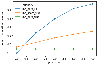
Next, let’s compare three quanitites across generations: - rho_beta_true, the correlation between true genetic effects for pheno_1 and pheno_2, which doesn’t vary over time - rho_score_true, the correlation between true polygenic scores for pheno_1 and pheno_2, which reflects changes in genetic architecture induced by xAM - rho_beta_HE, the HE-regression estimate of rho_beta_true, which is biased upwards under xAM

results = pd.DataFrame.from_records([{'generation':key,
  'rho_beta_HE':value['HE_regression']['corr_HE'].iloc[1,0],
  'rho_score_true':value['sample_statistics']['vcov'].iloc[1,0],
  'rho_beta_true':sim.architecture.components[0].true_rho_beta[1,0]} for key,value in sim.results_store.items()]
                         )

pdat = pd.melt(results, id_vars='generation', var_name='quantity',
               value_name='genetic correlation measure')
sns.lineplot(data=pdat,
           x='generation',
           y='genetic correlation measure',
           hue='quantity',)
sns.scatterplot(data=pdat,
           x='generation',
           y='genetic correlation measure',
           hue='quantity',legend=False)

<Axes: xlabel='generation', ylabel='genetic correlation measure'>

Writing output to disk

We save the generation 4 genotypes to disk. Here, we write to zarr, an efficient parallel format ideal for cases where we’d like to reload the data into python, but also to the plink binary format:

xft.io.write_to_plink1(sim.haplotypes, '/tmp/plink_output')

/home/rsb/Dropbox/ftsim/xftsim/xftsim/io.py:194: UserWarning: Writing to the plink bfile format removes phase information
  warnings.warn("Writing to the plink bfile format removes phase information")
Writing BED: 100%|████████████████████████████████████████████████████████████████████████████████████████████████████████████████████████████████████████████████████████████████████| 1/1 [00:00<00:00,  9.34it/s]

Writing FAM... done.
Writing BIM... done.

/home/rsb/miniconda3/lib/python3.9/site-packages/pandas_plink/_write.py:261: FutureWarning: the 'line_terminator'' keyword is deprecated, use 'lineterminator' instead.
  df.to_csv(
/home/rsb/miniconda3/lib/python3.9/site-packages/pandas_plink/_write.py:288: FutureWarning: the 'line_terminator'' keyword is deprecated, use 'lineterminator' instead.
  df.to_csv(

xft.io.save_haplotype_zarr(sim.haplotypes, '/tmp/zarr_output', mode='w')

We can convert the phenotypes to Pandas dataframes, which we can then save using any method we like:

pheno_df = sim.phenotypes.xft.as_pd()
pheno_df

		phenotype_name	pheno_1	pheno_2	pheno_1	pheno_2	pheno_1	pheno_2
		component_name	additiveGenetic	additiveGenetic	additiveNoise	additiveNoise	phenotype	phenotype
		vorigin_relative	proband	proband	proband	proband	proband	proband
iid	fid	sex
4_0	4_0	0	-1.966416	-1.934732	-0.002914	-0.362107	-1.969329	-2.296839
4_1	4_0	0	-2.926725	-1.776690	0.189355	0.207299	-2.737370	-1.569391
4_2	4_1	0	-1.092239	-1.597979	1.325921	0.199160	0.233683	-1.398819
4_3	4_1	0	-0.711714	-1.140154	-0.652625	1.048390	-1.364339	-0.091765
4_4	4_2	0	-0.574885	-0.999057	-0.593752	-0.475246	-1.168637	-1.474302
...	...	...	...	...	...	...	...	...
4_7995	4_3997	1	1.663567	1.608789	1.210872	0.930285	2.874439	2.539074
4_7996	4_3998	0	1.173014	0.511302	1.246304	-0.215005	2.419319	0.296297
4_7997	4_3998	1	1.179811	1.610954	-0.950225	0.467568	0.229586	2.078522
4_7998	4_3999	0	0.418514	1.636576	-0.764532	-0.758268	-0.346019	0.878308
4_7999	4_3999	0	2.185312	1.953812	0.093433	0.410642	2.278744	2.364453

8000 rows × 6 columns

pheno_df.to_csv('/tmp/pheno_out.csv')