Simulating mating

Mating regimes (xftsim.mate.MatingRegime) serve two primary functions:

1. the mates per female the number and offspring count / sex per mating

2. deciding who mates with whom

Mating and offspring counts

The first (the mates per female the number and offspring count / sex per mating) is determined by the following arguments to the MatingRegime constructor:

• mates_per_female - the number of mating partners per female

• offspring_per_pair - the number of offspring per mate pair

• female_offspring_per_pair - the number of female offspring per mate pair

Each of this can be constant or variable.

Variable counts

xftsim.utils provides the VariableCount class for random counts which include a draw method for generating random variates, an expectation property that returns the expected value, and a nonzero_fraction property that returns the expected number of nonzero counts. The later is useful for determining, e.g., the fraction of couples expected to produce offspring.

The simplest VariableCount subclass is the ConstantCount:

import xftsim as xft

ccount = xft.utils.ConstantCount(2)
ccount.draw(3), ccount.expectation, ccount.nonzero_fraction

(array([2, 2, 2]), 2, 1.0)

Other useful VariableCount subclasses are demonstrated below:

pcount = xft.utils.PoissonCount(2)
nbcount = xft.utils.NegativeBinomialCount(2,.5)
ztpcount = xft.utils.ZeroTruncatedPoissonCount(2)
mixcount = xft.utils.MixtureCount(componentCounts=[xft.utils.ConstantCount(0),
                                                   xft.utils.ConstantCount(3)],
                                  mixture_probabilities= [.4,.6])

for count in [pcount, nbcount, ztpcount, mixcount]:
    print(count.expectation, count.nonzero_fraction)

2 0.8646647167633873
2.0 0.75
2.3130352854993315 1
1.7999999999999998 0.6

Who with whom?

The second (who mates with whom) is mostly determined by the .mate() method of the MatingRegime but also by two boolean flags provided to the MatingRegime constructor:

• sex_aware if True, enforces a regime where males may only mate with females and vice versa. In many cases, we have no interest in sex effects and it is therefore convenient to set this to False to increase the effective population size.

• exhaustive if False when assigning mates, male mates are sampled with replacement. This too is convenient to set to False but should have little impact either way in sufficiently large simulations.

The mate() methods are specific each MatingRegime subclass. Generally speaking, they map haplotype and phenotype arrays to a MateAssignment object.

In what follows, we first introduce simple random mating regimes, then MateAssignment objects, and finally we’ll move on to more complex mating regimes.

Throughout, we’ll reference the toy dataset below:

import xftsim as xft

demo = xft.sim.DemoSimulation('BGRM')
demo

<DemoSimulation>
Bivariate GCTA with balanced random mating demo

n = 2000; m = 400
Two phenotypes, height and bone mineral denisty (BMD)
assuming bivariate GCTA infinitessimal archtecture
with h2 values set to 0.5 and 0.4 for height and BMD
respectively and a genetic effect correlation of 0.0.

Random mating

The simplest mating regime is that of random mating.

from xftsim.mate import RandomMatingRegime
from xftsim.utils import ConstantCount, PoissonCount

rm_regime = RandomMatingRegime(offspring_per_pair = ConstantCount(2),
                                mates_per_female = ConstantCount(1),
                                female_offspring_per_pair = 'balanced',
                                sex_aware = False,
                                exhaustive = True)

Setting female_offspring_per_pair to "balanced" rather than a VariableCount object will result in a equal number of male and female offspring.

It is sometimes useful to predict how the population size will change across generations. The MatingRegime.population_growth_factor property reveals the expected multiplicative change in population size each generation.

As we specified rm_regime such that each female is paired with exactly one male and each mating will produce exactly one offspring, we expect constant population size:

rm_regime.population_growth_factor

1.0

Of course, this is not always the case, as we demonstrate below:

rm_regime2 = RandomMatingRegime(offspring_per_pair = PoissonCount(2.2),
                                mates_per_female = PoissonCount(1.1),
                                female_offspring_per_pair = 'balanced',
                                sex_aware = False,
                                exhaustive = True)

rm_regime2.population_growth_factor

1.2100000000000002

Mate assignments

Mating regime objects map haplotypes and phenotypes to a MateAssignment object, which stores information about who mates with whom and the offspring such matings produce:

In practice, users will rarely call MateAssignment.mate() directly as this occurs automatically when running a simulation.

mate_assignment = rm_regime.mate(haplotypes=demo.haplotypes,
                                 phenotypes=demo.phenotypes)

Since the mating regime we’re using is random, the only information the mate method uses from either the haplotypes or phenotypes would be the associated index.SampleIndex object.

Two useful perspectives for viewing a MateAssignment are the mating_frame, which is indexed by couple, and the reproduction_frame, which is indexed by offspring:

mate_assignment.get_mating_frame()

	maternal_sample	maternal_iid	maternal_fid	maternal_sex	paternal_sample	paternal_iid	paternal_fid	paternal_sex	n_offspring	n_female_spring
0	0..1_1980.1_990	1_1980	1_990	1	0..1_321.1_160	1_321	1_160	1	2	0
1	0..1_782.1_391	1_782	1_391	0	0..1_1766.1_883	1_1766	1_883	0	2	1
2	0..1_1899.1_949	1_1899	1_949	1	0..1_772.1_386	1_772	1_386	0	2	2
3	0..1_229.1_114	1_229	1_114	1	0..1_1129.1_564	1_1129	1_564	1	2	1
4	0..1_1260.1_630	1_1260	1_630	1	0..1_1745.1_872	1_1745	1_872	1	2	1
...	...	...	...	...	...	...	...	...	...	...
995	0..1_912.1_456	1_912	1_456	0	0..1_430.1_215	1_430	1_215	1	2	2
996	0..1_1892.1_946	1_1892	1_946	1	0..1_838.1_419	1_838	1_419	1	2	0
997	0..1_642.1_321	1_642	1_321	0	0..1_260.1_130	1_260	1_130	0	2	2
998	0..1_75.1_37	1_75	1_37	1	0..1_1063.1_531	1_1063	1_531	1	2	1
999	0..1_425.1_212	1_425	1_212	1	0..1_1697.1_848	1_1697	1_848	1	2	2

1000 rows × 10 columns

mate_assignment.get_reproduction_frame()

	iid	fid	sex	maternal_sample	maternal_iid	maternal_fid	maternal_sex	paternal_sample	paternal_iid	paternal_fid	paternal_sex
sample
0..2_0.2_0	2_0	2_0	1	0..1_1980.1_990	1_1980	1_990	1	0..1_321.1_160	1_321	1_160	1
0..2_1.2_0	2_1	2_0	1	0..1_1980.1_990	1_1980	1_990	1	0..1_321.1_160	1_321	1_160	1
0..2_2.2_1	2_2	2_1	0	0..1_782.1_391	1_782	1_391	0	0..1_1766.1_883	1_1766	1_883	0
0..2_3.2_1	2_3	2_1	1	0..1_782.1_391	1_782	1_391	0	0..1_1766.1_883	1_1766	1_883	0
0..2_4.2_2	2_4	2_2	0	0..1_1899.1_949	1_1899	1_949	1	0..1_772.1_386	1_772	1_386	0
...	...	...	...	...	...	...	...	...	...	...	...
0..2_1995.2_997	2_1995	2_997	0	0..1_642.1_321	1_642	1_321	0	0..1_260.1_130	1_260	1_130	0
0..2_1996.2_998	2_1996	2_998	0	0..1_75.1_37	1_75	1_37	1	0..1_1063.1_531	1_1063	1_531	1
0..2_1997.2_998	2_1997	2_998	1	0..1_75.1_37	1_75	1_37	1	0..1_1063.1_531	1_1063	1_531	1
0..2_1998.2_999	2_1998	2_999	0	0..1_425.1_212	1_425	1_212	1	0..1_1697.1_848	1_1697	1_848	1
0..2_1999.2_999	2_1999	2_999	0	0..1_425.1_212	1_425	1_212	1	0..1_1697.1_848	1_1697	1_848	1

2000 rows × 11 columns

Nonrandom mating regimes

It will be challenging to to understand this information if you haven’t read the tutorial on indexing! Specifically, understanding xftsim.index.ComponentIndex is essential.

As xftsim mating regimes are privy to haplotypes and phenotypes, the can be very general. Here we present a few commonly used regimes.

Linear assortative mating

By “linear assortative mating”, we refer to mating mediated through a linear combination of phenotypic components. An exchangeable linear regime is provided by xft.mate.LinearAssortativeMatingRegime. Concretely, assume we want an exchangeable regime for \(k\) phenotypes with cross-mate correlations fixed at r. That is, given female and male phenotypes \(Y,\tilde{Y}\in R^{n\times k}\), respectively, this regime will generate a mating permutation \(P\)

such that the empirical correlation is

\[\text{corr}(Y,P\tilde{Y})\approx r\cdot1_{k\times k}.\]

Univariate primary phenotypic assortment

We can implement univariate assortative mating mediated through a single phenotype via LinearAssortativeMatingRegime. Below we do this for height, setting the cross-mate correlation to 0.5. We iterate for a single generation and then observe the sample mating statstics:

from xftsim.mate import LinearAssortativeMatingRegime

reg_pp = LinearAssortativeMatingRegime(r=.5,
    component_index=xft.index.ComponentIndex.from_product(phenotype_name='height',
                                                          component_name='phenotype'))

demo_pp = xft.sim.DemoSimulation()
demo_pp.mating_regime = reg_pp
demo_pp.run(1)
xmate_corr = demo_pp.results['mating_statistics']['mate_correlations']
xmate_corr.iloc[:xmate_corr.shape[0]//2,xmate_corr.shape[0]//2:]

component	height.additiveGenetic.father	BMD.additiveGenetic.father	height.additiveNoise.father	BMD.additiveNoise.father	height.phenotype.father	BMD.phenotype.father
component
height.additiveGenetic.mother	0.268342	-0.008584	0.285039	-0.048256	0.397498	-0.042764
BMD.additiveGenetic.mother	0.008731	-0.046509	-0.004701	0.030176	0.002762	-0.003530
height.additiveNoise.mother	0.213312	0.011146	0.245511	0.047010	0.329757	0.043285
BMD.additiveNoise.mother	0.025006	0.073521	0.004836	-0.003132	0.021229	0.040452
height.phenotype.mother	0.345829	0.001849	0.380946	-0.000849	0.522178	0.000415
BMD.phenotype.mother	0.024631	0.029059	0.000926	0.015699	0.018117	0.029240

Univariate social / genetic homogamy

Social or genetic homogamy can be modeled by specifying that mating operates only on the non-heritable or heritable components respectively:

from xftsim.mate import LinearAssortativeMatingRegime

reg_social = LinearAssortativeMatingRegime(r=.5,
    component_index=xft.index.ComponentIndex.from_product(phenotype_name='height',
                                                          component_name='additiveNoise'))

reg_genetic = LinearAssortativeMatingRegime(r=.5,
    component_index=xft.index.ComponentIndex.from_product(phenotype_name='height',
                                                          component_name='additiveGenetic'))


demo_soc = xft.sim.DemoSimulation(); demo_gen = xft.sim.DemoSimulation()
demo_soc.mating_regime = reg_social; demo_gen.mating_regime = reg_genetic;
demo_soc.run(1); demo_gen.run(1)
xmate_corr_soc = demo_soc.results['mating_statistics']['mate_correlations']
xmate_corr_soc.iloc[:xmate_corr_soc.shape[0]//2,xmate_corr_soc.shape[0]//2:]

component	height.additiveGenetic.father	BMD.additiveGenetic.father	height.additiveNoise.father	BMD.additiveNoise.father	height.phenotype.father	BMD.phenotype.father
component
height.additiveGenetic.mother	-0.075997	0.020729	-0.022070	-0.009579	-0.068682	0.006065
BMD.additiveGenetic.mother	-0.034681	0.001651	-0.049497	-0.010576	-0.058171	-0.006805
height.additiveNoise.mother	0.048020	0.039968	0.497350	-0.017413	0.372348	0.012479
BMD.additiveNoise.mother	0.024209	-0.048029	-0.028814	0.026596	-0.002513	-0.010783
height.phenotype.mother	-0.020428	0.043707	0.341454	-0.019438	0.217930	0.013352
BMD.phenotype.mother	-0.003607	-0.034945	-0.052617	0.013294	-0.038352	-0.012345

xmate_corr_gen = demo_gen.results['mating_statistics']['mate_correlations']
xmate_corr_gen.iloc[:xmate_corr_gen.shape[0]//2,xmate_corr_gen.shape[0]//2:]

component	height.additiveGenetic.father	BMD.additiveGenetic.father	height.additiveNoise.father	BMD.additiveNoise.father	height.phenotype.father	BMD.phenotype.father
component
height.additiveGenetic.mother	0.529864	0.001163	0.063315	0.035746	0.415366	0.028550
BMD.additiveGenetic.mother	-0.004869	-0.007057	-0.030289	0.034901	-0.024318	0.022398
height.additiveNoise.mother	-0.027741	-0.006710	0.006791	0.031207	-0.014773	0.019760
BMD.additiveNoise.mother	-0.004571	-0.025001	0.045424	0.011315	0.028142	-0.007923
height.phenotype.mother	0.365798	-0.003683	0.050528	0.046995	0.291459	0.034050
BMD.phenotype.mother	-0.006635	-0.024104	0.016955	0.030649	0.007047	0.007698

Exchangeable bivariate phenotypic assortment

Exchangeable bivariate phenotypic assortment is also easily accommodated in this framework. Here we implement such a regime for \(r\)=.1 across height and bone mineral density (BMD):

reg_biv = LinearAssortativeMatingRegime(r=.1,
    component_index=xft.index.ComponentIndex.from_product(phenotype_name=['height','BMD'],
                                                          component_name='phenotype'))

demo_biv = xft.sim.DemoSimulation()
demo_biv.mating_regime = reg_biv
demo_biv.run(1)
xmate_corr = demo_biv.results['mating_statistics']['mate_correlations']
xmate_corr.iloc[:xmate_corr.shape[0]//2,xmate_corr.shape[0]//2:]

component	height.additiveGenetic.father	BMD.additiveGenetic.father	height.additiveNoise.father	BMD.additiveNoise.father	height.phenotype.father	BMD.phenotype.father
component
height.additiveGenetic.mother	0.042121	0.007638	0.063715	0.064258	0.076388	0.054666
BMD.additiveGenetic.mother	0.011518	-0.000970	0.025269	0.016718	0.026438	0.012362
height.additiveNoise.mother	-0.005662	0.005028	0.117724	0.087100	0.079050	0.070748
BMD.additiveNoise.mother	0.023836	0.056490	0.033903	0.063639	0.041705	0.084921
height.phenotype.mother	0.025256	0.008798	0.126190	0.105230	0.108031	0.087188
BMD.phenotype.mother	0.026047	0.044510	0.042460	0.060993	0.049401	0.075330

Generalized assortive mating

We can also model general assortment to achieve an arbitrary cross-mate cross-correlation matrix across a set of \(K\) phenotypes. In xftsim this is done by solving an equivalent corresponding combinatorial optimization problem. This problem (the quadratic assignment problem (QAP)) is NP-hard and requires the use of the closed-source LocalSolver software and corresponding Python library.

The LocalSolver dependences must be installed separately. Additionally, a license is required to run the software. Academic licenses are available from the LocalSolver website.

Suppose we want to model complex assortment across BMI, height, years of education, and smoking behaviors. In the UK Biobank, these traits have approximately the following cross-mate cross-correlation structure (see fig 1, Border et al. 2022):

\[\begin{split}\begin{array}{c|cccc} & \text{BMI} & \text{height} & \text{edu} & \text{smoke}\\ \hline \text{BMI} & +.26\\ \text{height} & -.05 & +.24\\ \text{edu} & -.11 & +.10 & +.33\\ \text{smoke} & +.08 & -.02 & -.06 & +.19 \end{array}\end{split}\]

To model this in xftsim we can use GeneralAssortativeMatingRegime:

import xftsim as xft
import numpy as np
import matplotlib.pyplot as plt
plt.rcParams['figure.dpi'] = 240 ## better looking plots
plt.rcParams['figure.figsize'] = [6.,4.]
xft.config.print_durations_threshold = 1. ## reduce output verbosity

cind = xft.index.ComponentIndex.from_product(['bmi','height','edu','smoke'],
                                             'phenotype')

xmatecorr = np.array([[.26,-.05,-.11, .08],
                      [-.05,.24,.10,-.02],
                      [-.11,.10,.33,-.06],
                      [.08,-.02,-.06,.19]])



mate_reg = xft.mate.GeneralAssortativeMatingRegime(component_index=cind,
    cross_corr=xmatecorr,
    control=dict(nb_threads=8,
                 time_limit = 120,
                 time_between_displays=5))

Solving the combinatorial optimization required for arbitrary cross-trait assortative mating can be computationally intensive. Finding the optimal solution is NP-hard, but we can do pretty well by iterating for a fixed amount of time. This time limit (specified above by the time_limit key in the control dictionary) is sensitive to both the population size and number of phenotypes under assortment. We suggest experimentation, comparing the realized cross-mate correlation matrix to the target matrix. Further, it is often faster to batch mating for computational efficiency (see the section on batched regimes below).

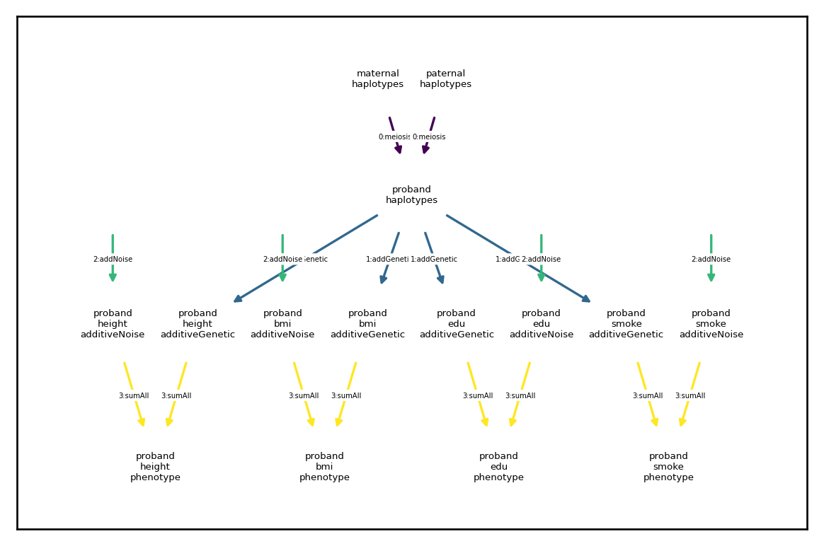
To demonstrate this regime, we will assume an independent infinitessimal model with the following (arbitrary) panmictic heritabilities: \(h^2_\text{BMI} = .4\), \(h^2_\text{height} = .6\), \(h^2_\text{edu} = .3\), \(h^2_\text{smoke} = .25\) and first specify the corresponding phenogenetic architecture:

n=2000; m=800
h2=np.array([.4, .6, .3, .25])

# founder haplotypes
haplotypes = xft.founders.founder_haplotypes_uniform_AFs(n=n,m=m)
# recombination map
rmap = xft.reproduce.RecombinationMap.constant_map_from_haplotypes(p=.1,
                                                                   haplotypes=haplotypes)
# additive phenogenetic architecture
arch = xft.arch.GCTA_Architecture(h2=h2,
                                  phenotype_name=['bmi','height','edu','smoke'],
                                  haplotypes=haplotypes)
# simulation object
sim = xft.sim.Simulation(founder_haplotypes=haplotypes,
                         recombination_map=rmap,
                         architecture=arch,
                         mating_regime = mate_reg,
                         statistics= [xft.stats.SampleStatistics(),
                                      xft.stats.MatingStatistics()])
arch.draw_dependency_graph(font_size=4)

sim.run(1)

    2.35 mks in increment_generation
    6.40 mks in reproduce
  172.60 ms in compute_phenotypes
Push initial solution 100%
Model:  expressions = 6006012, decisions = 1, constraints = 1, objectives = 1
Param:  time limit = 120 sec, no iteration limit, nb threads = 8
        time between displays = 5

[objective direction ]:     minimize

[  0 sec,       0 itr]:     0.904413
[ optimality gap     ]:       > 100%
[  5 sec,      88 itr]:     0.183807
[ 10 sec,     182 itr]:     0.144635
[ 15 sec,     278 itr]:      0.11705
[ 20 sec,     367 itr]:    0.0850189
[ 25 sec,     429 itr]:    0.0621292
[ 30 sec,     517 itr]:    0.0507904
[ 35 sec,     604 itr]:    0.0432865
[ 40 sec,     694 itr]:    0.0361864
[ 45 sec,     811 itr]:    0.0276867
[ 50 sec,     893 itr]:    0.0217341
[ optimality gap     ]:       > 100%
[ 55 sec,     979 itr]:    0.0171043
[ 60 sec,    1067 itr]:    0.0147058
[ 65 sec,    1165 itr]:    0.0108805
[ 70 sec,    1261 itr]:    0.0101373
[ 75 sec,    1336 itr]:   0.00932477
[ 80 sec,    1420 itr]:   0.00825076
[ 85 sec,    1526 itr]:   0.00698871
[ 90 sec,    1619 itr]:   0.00528569
[ 95 sec,    1707 itr]:   0.00486376
[100 sec,    1788 itr]:   0.00465838
[ optimality gap     ]:       > 100%
[105 sec,    1869 itr]:   0.00435036
[110 sec,    2007 itr]:   0.00360183
[115 sec,    2148 itr]:   0.00340868
[120 sec,    2280 itr]:   0.00330814
[120 sec,    2280 itr]:   0.00330814
[ optimality gap     ]:       > 100%

2280 iterations performed in 120 seconds

Feasible solution: 
  obj    =   0.00330814
  gap    =       > 100%
  bounds =     -36.9987
  138.53 s in mate
    1.89 mks in update_pedigree
   14.40 ms in sample statistics
   42.58 ms in mating statistics
   57.05 ms in estimate_statistics
    2.23 mks in process
  138.76 s in run_generation
  138.76 s in run

Comparing our realized mating structure to the target shows that the optimzation completed successfully:

sim.results['mating_statistics']['mate_correlations'].iloc[:4,4:]

component	bmi.phenotype.father	height.phenotype.father	edu.phenotype.father	smoke.phenotype.father
component
bmi.phenotype.mother	0.259063	-0.050205	-0.108674	0.076731
height.phenotype.mother	-0.045843	0.243643	0.100098	-0.022487
edu.phenotype.mother	-0.106854	0.093305	0.326693	-0.057785
smoke.phenotype.mother	0.081431	-0.023318	-0.059520	0.190134

xmatecorr

array([[ 0.26, -0.05, -0.11,  0.08],
       [-0.05,  0.24,  0.1 , -0.02],
       [-0.11,  0.1 ,  0.33, -0.06],
       [ 0.08, -0.02, -0.06,  0.19]])

Batched mating regimes

A xft.mate.BatchedMatingRegime simply takes an existing mating regime and applies in to subsets of the data. By default, it will split the sample into equal random subsamples no larger than max_batch_size. This can be very useful in combination with xft.mate.GeneralAssortativeMatingRegime as it’s often faster to solve multiple smaller optimization problems than one large problem. Here we achieve similar results to the previous example by optimizing for 30 seconds (twice) in each half of a random split of the data as opposed to 120 seconds in the full sample.

mate_batch = xft.mate.GeneralAssortativeMatingRegime(component_index=cind,
    cross_corr=xmatecorr,
    control=dict(nb_threads=8,
                 time_limit = 30,
                 time_between_displays=5))

batched_regime = xft.mate.BatchedMatingRegime(mate_batch,
                                              max_batch_size=1000)

sim = xft.sim.Simulation(founder_haplotypes=haplotypes,
                         recombination_map=rmap,
                         architecture=arch,
                         mating_regime = batched_regime,
                         statistics= [xft.stats.SampleStatistics(),
                                      xft.stats.MatingStatistics()])
sim.run(1)

    2.91 mks in increment_generation
    2.78 mks in reproduce
   66.91 ms in compute_phenotypes
Push initial solution 100%
Model:  expressions = 1503012, decisions = 1, constraints = 1, objectives = 1
Param:  time limit = 30 sec, no iteration limit, nb threads = 8
        time between displays = 5

[objective direction ]:     minimize

[  0 sec,       0 itr]:     0.849955
[ optimality gap     ]:       > 100%
[  5 sec,     502 itr]:    0.0316502
[ 10 sec,    1019 itr]:   0.00943589
[ 15 sec,    1545 itr]:   0.00598421
[ 20 sec,    2181 itr]:   0.00537489
[ 25 sec,    2756 itr]:   0.00524854
[ 30 sec,    3412 itr]:    0.0051854
[ 30 sec,    3412 itr]:    0.0051854
[ optimality gap     ]:       > 100%

3412 iterations performed in 30 seconds

Feasible solution: 
  obj    =    0.0051854
  gap    =       > 100%
  bounds =     -32.7763
Push initial solution 100%
Model:  expressions = 1503012, decisions = 1, constraints = 1, objectives = 1
Param:  time limit = 30 sec, no iteration limit, nb threads = 8
        time between displays = 5

[objective direction ]:     minimize

[  0 sec,       0 itr]:     0.990215
[ optimality gap     ]:       > 100%
[  5 sec,     493 itr]:    0.0100217
[ 10 sec,    1067 itr]:  -0.00687622
[ 15 sec,    1650 itr]:   -0.0106121
[ 20 sec,    2261 itr]:   -0.0121135
[ 25 sec,    2856 itr]:   -0.0125204
[ 30 sec,    3555 itr]:   -0.0126443
[ 30 sec,    3555 itr]:   -0.0126443
[ optimality gap     ]:       99.96%

3555 iterations performed in 30 seconds

Feasible solution: 
  obj    =   -0.0126443
  gap    =       99.96%
  bounds =     -30.9948
   67.65 s in mate
    2.07 mks in update_pedigree
   13.47 ms in sample statistics
   37.31 ms in mating statistics
   50.85 ms in estimate_statistics
    1.98 mks in process
   67.77 s in run_generation
   67.77 s in run

sim.results['mating_statistics']['mate_correlations'].iloc[:4,4:]

component	bmi.phenotype.father	height.phenotype.father	edu.phenotype.father	smoke.phenotype.father
component
bmi.phenotype.mother	0.259715	-0.050911	-0.107914	0.077503
height.phenotype.mother	-0.047922	0.239276	0.099072	-0.016085
edu.phenotype.mother	-0.107737	0.096561	0.325611	-0.060520
smoke.phenotype.mother	0.080135	-0.021780	-0.057260	0.190545

xmatecorr

array([[ 0.26, -0.05, -0.11,  0.08],
       [-0.05,  0.24,  0.1 , -0.02],
       [-0.11,  0.1 ,  0.33, -0.06],
       [ 0.08, -0.02, -0.06,  0.19]])

Again, we have satisfactorily reproduced the target cross-mate correlation structure. This batched approach is likely the only practical way to proceed for generalized assortative mating in larger samples.