Phenogenetic architectures
Overview
Here’s where things start to get interesting. The ability to easily construct and modify phenogenetic architectures with arbitrary complexity was the core motivating feature underlying the development of xftsim. In what follows, we introduce the ArchitectureComponent and Architecture classes that make this possible.
ArchitectureComponent objects
An Architecture object largely consists of an iterable collection of ArchitectureComponents. These component objects take haplotype and phenotype data as inputs and modify phenotypes by reference. For example, the widely used additive genetic architecture
is represented in xftsim as a collection of three components: the additive genetic component \(X\beta\), the additive noise component \(e\), and the sum transformation \(y = X\beta + e\).
[106]:
import numpy as np
import xftsim as xft
import matplotlib.pyplot as plt
plt.rcParams['figure.dpi'] = 240 ## better looking plots
plt.rcParams['figure.figsize'] = [6.,4.]
np.random.seed(123)

demo = xft.sim.DemoSimulation("BGRM")
demo
[106]:
<DemoSimulation>
Bivariate GCTA with balanced random mating demo

n = 2000; m = 400
Two phenotypes, height and bone mineral denisty (BMD)
assuming bivariate GCTA infinitessimal archtecture
with h2 values set to 0.5 and 0.4 for height and BMD
respectively and a genetic effect correlation of 0.0.
This architecture consists of three components:
[107]:
len(demo.architecture.components)
[107]:
3
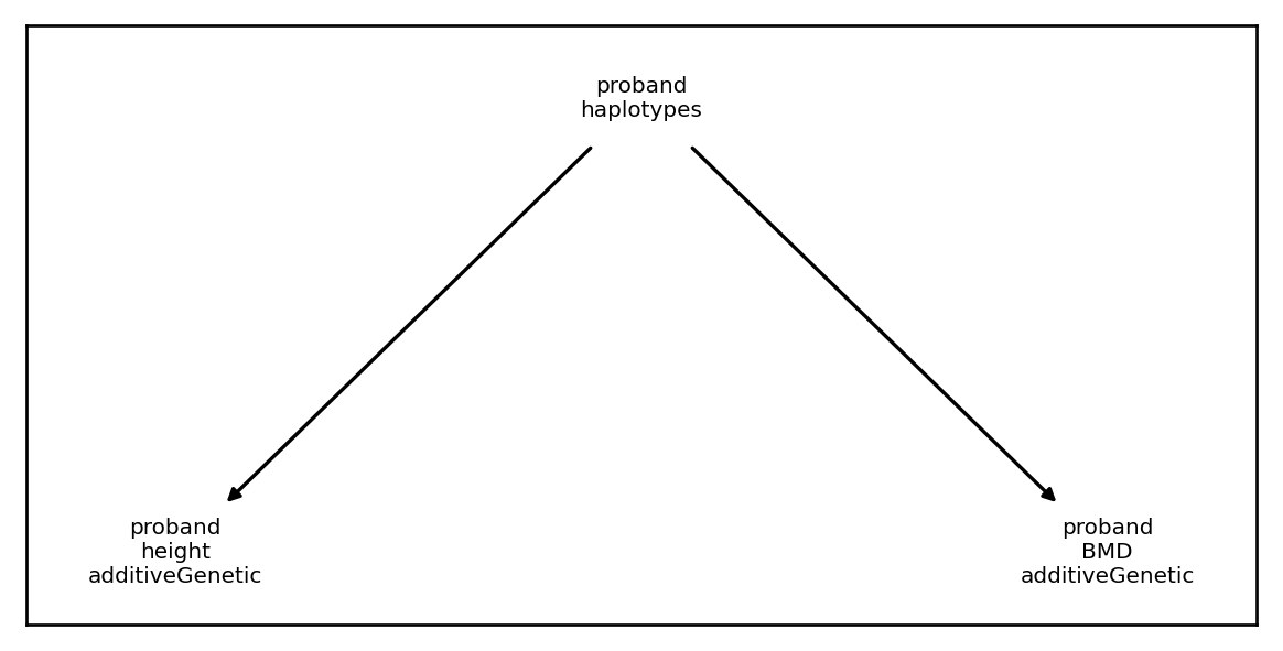
The genetic component uses haplotype information (but not phenotype information) as inputs and generates the additiveGenetic phenotype component as its output:
[108]:
demo.architecture.components[0]
[108]:
<class 'xftsim.arch.AdditiveGeneticComponent'>

## INPUTS:
 - haplotypes: True
 - phenotype components:
<Empty ComponentIndex>

## OUTPUTS:
 - phenotype components:
<ComponentIndex>
  1 component of 2 phenotypes spanning 1 generation
                               phenotype_name   component_name  \
component
height.additiveGenetic.proband         height  additiveGenetic
BMD.additiveGenetic.proband               BMD  additiveGenetic

                                vorigin_relative     comp_type
component
height.additiveGenetic.proband                -1  intermediate
BMD.additiveGenetic.proband                   -1  intermediate
The noise component, on the other hand, doesn’t use haplotype information or phenotype information as inputs and generates the additiveNoise phenotype component as its output:
[109]:
demo.architecture.components[1]
[109]:
<class 'xftsim.arch.AdditiveNoiseComponent'>

## INPUTS:
 - haplotypes: False
 - phenotype components:
<Empty ComponentIndex>

## OUTPUTS:
 - phenotype components:
<ComponentIndex>
  1 component of 2 phenotypes spanning 1 generation
                             phenotype_name component_name  vorigin_relative  \
component
height.additiveNoise.proband         height  additiveNoise                -1
BMD.additiveNoise.proband               BMD  additiveNoise                -1

                                 comp_type
component
height.additiveNoise.proband  intermediate
BMD.additiveNoise.proband     intermediate
Finally, the sum component ignores haplotype data but uses both the additiveGenetic and additiveNoise components to compute the phenotype component:
[110]:
demo.architecture.components[2]
[110]:
<class 'xftsim.arch.SumAllTransformation'>

## INPUTS:
 - haplotypes: False
 - phenotype components:
<ComponentIndex>
  2 components of 2 phenotypes spanning 1 generation
                               phenotype_name   component_name  \
component
height.additiveGenetic.proband         height  additiveGenetic
height.additiveNoise.proband           height    additiveNoise
BMD.additiveGenetic.proband               BMD  additiveGenetic
BMD.additiveNoise.proband                 BMD    additiveNoise

                                vorigin_relative     comp_type
component
height.additiveGenetic.proband                -1  intermediate
height.additiveNoise.proband                  -1  intermediate
BMD.additiveGenetic.proband                   -1  intermediate
BMD.additiveNoise.proband                     -1  intermediate

## OUTPUTS:
 - phenotype components:
<ComponentIndex>
  1 component of 2 phenotypes spanning 1 generation
                         phenotype_name component_name  vorigin_relative  \
component
height.phenotype.proband         height      phenotype                -1
BMD.phenotype.proband               BMD      phenotype                -1

                         comp_type
component
height.phenotype.proband   outcome
BMD.phenotype.proband      outcome
Dependency graphs
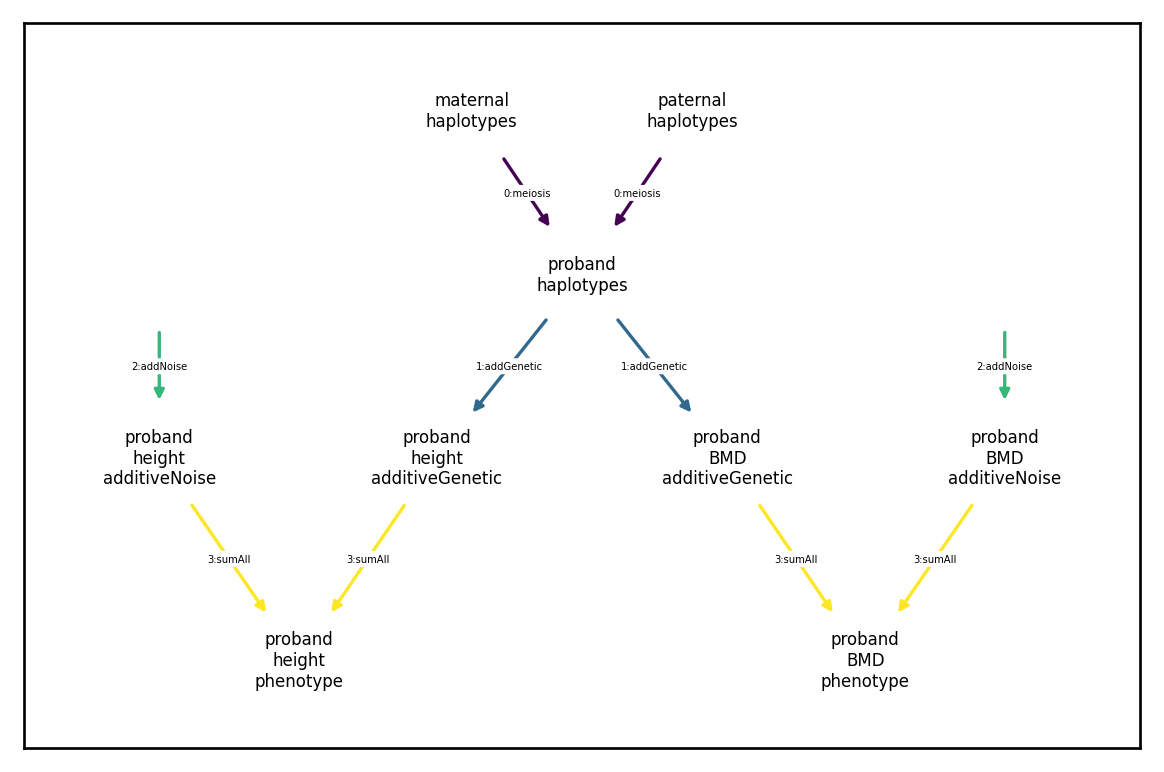
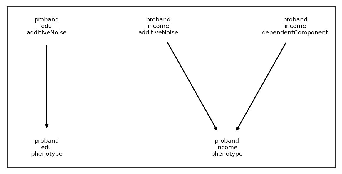
All ArchitectureComponent and Architecture objects include a draw_dependency_graph() method for visualizing the dependence between components. This can be helpful for making sure your model is correctly specified. For example, the SumAllTransformation above has the following dependency graph:
[112]:
plt.rcParams['figure.figsize'] = [6.,3.]
demo.architecture.components[2].draw_dependency_graph()
The Architecture object, which includes all three components has the following dependency graph:
[113]:
plt.rcParams['figure.figsize'] = [6.,4.]
demo.architecture.draw_dependency_graph()
We will go through some commonly used ArchitectureComponents (including the above) in what follows.
Genetic components
To specify an ‘arch.AdditiveGeneticComponent’, we need to first create an effect.AdditiveEffects object. Additive effects relating \(m\) diploid variants to \(k\) phenotypic components are comprised of an \(m\times k\) matrix of effects, an index of the \(m\) variants (can be xft.index.HaploidVariantIndex or xft.index.DiploidVariantIndex), and an index of the \(k\) components in the form of an xft.index.ComponentIndex.
For example, we can create effects under the additive model specified above as follows:
[114]:
import numpy as np

beta = np.random.randn(demo.haplotypes.xft.m, 1) * np.sqrt(.5)
vindex = demo.haplotypes.xft.get_variant_indexer()
cindex = xft.index.ComponentIndex.from_product('height', 'additiveGenetic')

effects = xft.effect.AdditiveEffects(beta=beta,
                                     variant_indexer=vindex,
                                     component_indexer=cindex)
Alternatively, we could construct additive components for two phenotypes, height and bone mineral density (BMD), with genetic variances 0.5 and 0.4, respectively, and genetic effect correlation 0.25 as follows:
[115]:
m = demo.haplotypes.xft.m
vcov = np.array([[.5, .25*np.sqrt(.5*.4)],
                 [.25*np.sqrt(.5*.4), .4]])


beta = np.random.multivariate_normal(mean = np.zeros(2),
                                     cov = vcov, size = m)
vindex = demo.haplotypes.xft.get_variant_indexer()
cindex = xft.index.ComponentIndex.from_product(('height','BMD'), 'additiveGenetic')

effects = xft.effect.AdditiveEffects(beta=beta,
                                     variant_indexer=vindex,
                                     component_indexer=cindex)
We can confirm that these effects behave as expected if desired:
[116]:
correlation_matrix = np.corrcoef(demo.haplotypes.data @ effects.beta_unscaled_unstandardized_haploid, rowvar=-False)
covariance_matrix = np.cov(demo.haplotypes.data @ effects.beta_unscaled_unstandardized_haploid, rowvar=-False)

correlation_matrix, covariance_matrix
[116]:
(array([[1.        , 0.32544254],
        [0.32544254, 1.        ]]),
 array([[0.49780155, 0.14565898],
        [0.14565898, 0.40241082]]))
We then pass the AdditiveEffects object to the AdditiveGeneticComponent constructor to generate the corresponding archetecture component:
[118]:
plt.rcParams['figure.figsize'] = [6.,3.]
arch = xft.arch.AdditiveGeneticComponent(effects)
arch.draw_dependency_graph()
arch
[118]:
<class 'xftsim.arch.AdditiveGeneticComponent'>

## INPUTS:
 - haplotypes: True
 - phenotype components:
<Empty ComponentIndex>

## OUTPUTS:
 - phenotype components:
<ComponentIndex>
  1 component of 2 phenotypes spanning 1 generation
                               phenotype_name   component_name  \
component
height.additiveGenetic.proband         height  additiveGenetic
BMD.additiveGenetic.proband               BMD  additiveGenetic

                                vorigin_relative     comp_type
component
height.additiveGenetic.proband                -1  intermediate
BMD.additiveGenetic.proband                   -1  intermediate
Noise components
Noise components are likely the simplest archetectural component to specify. For iid Gaussian noise, we only need to provide variances (or standard deviations if preferred) and the names of the corresponding phenotypes to the AdditiveNoiseComponent constructor. Here we construct independent noise components for height and BMD with variances 0.5 and 0.6, respectively:
[119]:
inoise = xft.arch.AdditiveNoiseComponent(variances=[.5,.6], phenotype_name=['height', 'BMD'])
inoise
[119]:
<class 'xftsim.arch.AdditiveNoiseComponent'>

## INPUTS:
 - haplotypes: False
 - phenotype components:
<Empty ComponentIndex>

## OUTPUTS:
 - phenotype components:
<ComponentIndex>
  1 component of 2 phenotypes spanning 1 generation
                             phenotype_name component_name  vorigin_relative  \
component
height.additiveNoise.proband         height  additiveNoise                -1
BMD.additiveNoise.proband               BMD  additiveNoise                -1

                                 comp_type
component
height.additiveNoise.proband  intermediate
BMD.additiveNoise.proband     intermediate
If we want (possibly correlated) multivariate normal noise components, we can use CorrelatedNoiseComponent instead. Here we set the correlation between the noise components for height and BMD to 0.3:
[120]:
vcov = np.array([[.5, .3*np.sqrt(.5*.6)],
                 [.3*np.sqrt(.5*.6), .6]])

cnoise = xft.arch.CorrelatedNoiseComponent(vcov=vcov, phenotype_name=['height', 'BMD'])
cnoise
[120]:
<class 'xftsim.arch.CorrelatedNoiseComponent'>

## INPUTS:
 - haplotypes: False
 - phenotype components:
<Empty ComponentIndex>

## OUTPUTS:
 - phenotype components:
<ComponentIndex>
  1 component of 2 phenotypes spanning 1 generation
                               phenotype_name   component_name  \
component
height.correlatedNoise.proband         height  correlatedNoise
BMD.correlatedNoise.proband               BMD  correlatedNoise

                                vorigin_relative     comp_type
component
height.correlatedNoise.proband                -1  intermediate
BMD.correlatedNoise.proband                   -1  intermediate
Causal dependencies
Univariate causal dependence
We use the term “causal dependences” to refer to scenarios where one phenotype component is directly affected by another within an individual. For example, suppose I want to model years of education and income. It may reasonable to assume that regardless whatever individual heritable and/or non-heritable influences on either outcome, years of education will have some possitve effect on income (i.e., advanced degrees increase earnings).
For simplicity, we will assume that neither trait is heritable, but that 50% of the variance in income is a linear function of years of education (which we treat here as continous for simplicity). I can model this dependence using LinearTransformationComponent.
One (very simple) generative model might look like this
First, we’ll model the independent parts of our phenotypes. We want education to be completely random so we’ll set it’s variance to 1.0, whereas the independent noise for income will have variance 0.5:
[121]:
ncomp = xft.arch.AdditiveNoiseComponent(variances=[1,.5],
                                        phenotype_name=['edu', 'income'])
ncomp
[121]:
<class 'xftsim.arch.AdditiveNoiseComponent'>

## INPUTS:
 - haplotypes: False
 - phenotype components:
<Empty ComponentIndex>

## OUTPUTS:
 - phenotype components:
<ComponentIndex>
  1 component of 2 phenotypes spanning 1 generation
                             phenotype_name component_name  vorigin_relative  \
component
edu.additiveNoise.proband               edu  additiveNoise                -1
income.additiveNoise.proband         income  additiveNoise                -1

                                 comp_type
component
edu.additiveNoise.proband     intermediate
income.additiveNoise.proband  intermediate
Next, we’ll add a LinearTransformationComponent, which requires the following arguments: - input_cindex: the ComponentIndex for the independent variable(s) - output_cindex: the ComponentIndex for the dependent variable(s) - coefficient_matrix: the matrix to premultiply the independent variables with to get the dependent variables - normalize: a boolean flag determining whether or not to standardize the independent variables prior to applying the linear transformation.
This will be very simple in this case as our matrix is 1x1:
[122]:
input_ind = xft.index.ComponentIndex(['edu'], ['additiveNoise'])
output_ind = xft.index.ComponentIndex(['income'], ['dependentComponent'])
coefficient_matrix = np.array([[np.sqrt(.5)]])

ccomp = xft.arch.LinearTransformationComponent(input_ind, output_ind,
                                               coefficient_matrix, normalize = True)
ccomp
[122]:
<LinearTransformationComponent>
                                           normalized_edu additiveNoise -1 intermediate
income_dependentComponent_-1_intermediate                                      0.707107
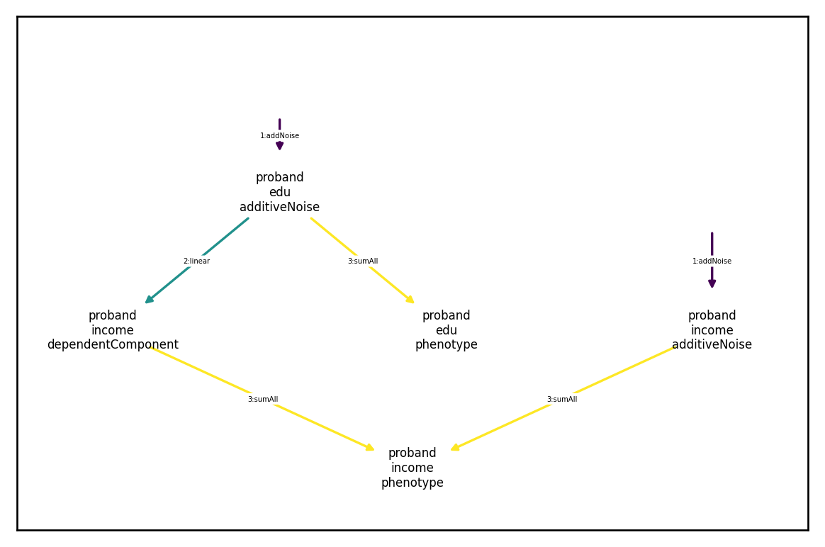
To put everything together, can add a SumAllTransformation, which we’ll cover in greater depth below:
[123]:
iind = xft.index.ComponentIndex(['edu','income','income'],
                                ['additiveNoise','additiveNoise','dependentComponent'])

strans = xft.arch.SumAllTransformation(input_cindex=iind)
strans.draw_dependency_graph()
strans
[123]:
<class 'xftsim.arch.SumAllTransformation'>

## INPUTS:
 - haplotypes: False
 - phenotype components:
<ComponentIndex>
  2 components of 2 phenotypes spanning 1 generation
                                  phenotype_name      component_name  \
component
edu.additiveNoise.proband                    edu       additiveNoise
income.additiveNoise.proband              income       additiveNoise
income.dependentComponent.proband         income  dependentComponent

                                   vorigin_relative     comp_type
component
edu.additiveNoise.proband                        -1  intermediate
income.additiveNoise.proband                     -1  intermediate
income.dependentComponent.proband                -1  intermediate

## OUTPUTS:
 - phenotype components:
<ComponentIndex>
  1 component of 2 phenotypes spanning 1 generation
                         phenotype_name component_name  vorigin_relative  \
component
edu.phenotype.proband               edu      phenotype                -1
income.phenotype.proband         income      phenotype                -1

                         comp_type
component
edu.phenotype.proband      outcome
income.phenotype.proband   outcome
Looking at the result, we see that everything is is as expected:
[125]:
plt.rcParams['figure.figsize'] = [6.,4.]
demo =  xft.sim.DemoSimulation()

test_sim = xft.sim.Simulation(founder_haplotypes=demo.haplotypes,
                              mating_regime=demo.mating_regime,
                              recombination_map= demo.recombination_map,
                              architecture = xft.arch.Architecture([ncomp, ccomp, strans]),
                              statistics=[xft.stats.SampleStatistics()],)

test_sim.architecture.draw_dependency_graph()
test_sim.run(1)
pd = test_sim.phenotypes.xft.as_pd()
pd.corr()**2
[125]:
| phenotype_name | edu | income | edu | income | |||
|---|---|---|---|---|---|---|---|
| component_name | additiveNoise | additiveNoise | dependentComponent | phenotype | phenotype | ||
| vorigin_relative | proband | proband | proband | proband | proband | ||
| phenotype_name | component_name | vorigin_relative | |||||
| edu | additiveNoise | proband | 1.000000 | 0.001337 | 1.000000 | 1.000000 | 0.525563 |
| income | additiveNoise | proband | 0.001337 | 1.000000 | 0.001337 | 0.001337 | 0.511000 |
| dependentComponent | proband | 1.000000 | 0.001337 | 1.000000 | 1.000000 | 0.525563 | |
| edu | phenotype | proband | 1.000000 | 0.001337 | 1.000000 | 1.000000 | 0.525563 |
| income | phenotype | proband | 0.525563 | 0.511000 | 0.525563 | 0.525563 | 1.000000 |
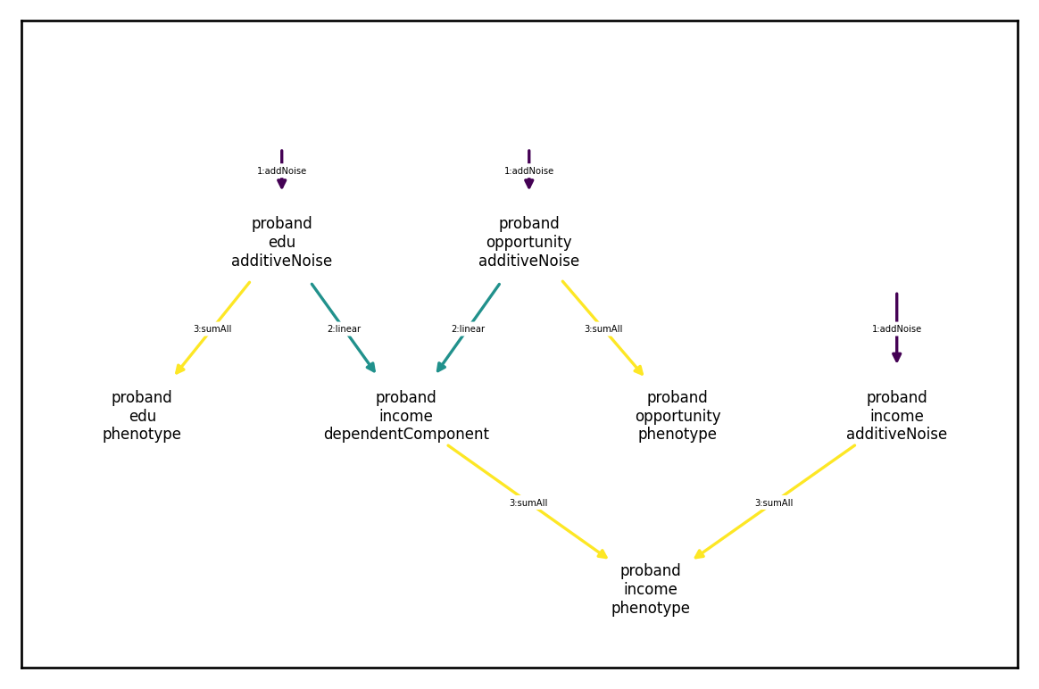
Multivariate causal dependence
No suppose we assume income is affected by not just a single education factor, but by education and some measure of “opportunity”.
Another simple model generative model might look like this
In this case, everything will be the same except that our linear transformation will be 2x1:
[126]:
ncomp = xft.arch.AdditiveNoiseComponent(variances=[1,1,.5],
                                        phenotype_name=['edu', 'opportunity', 'income'])
input_ind = xft.index.ComponentIndex(['edu','opportunity'], ['additiveNoise','additiveNoise'])
output_ind = xft.index.ComponentIndex(['income'], ['dependentComponent'])
coefficient_matrix = np.array([[np.sqrt(.25),np.sqrt(.25)]])

ccomp = xft.arch.LinearTransformationComponent(input_ind, output_ind,
                                               coefficient_matrix, normalize = True)
sind = xft.index.ComponentIndex(['edu','opportunity','income','income'],
                                ['additiveNoise','additiveNoise','additiveNoise','dependentComponent'])

strans = xft.arch.SumAllTransformation(input_cindex=sind)

test_sim = xft.sim.Simulation(founder_haplotypes=demo.haplotypes,
                              mating_regime=demo.mating_regime,
                              recombination_map= demo.recombination_map,
                              architecture = xft.arch.Architecture([ncomp, ccomp, strans]),
                              statistics=[xft.stats.SampleStatistics()],)

test_sim.architecture.draw_dependency_graph()
test_sim.run(1)
pd = test_sim.phenotypes.xft.as_pd()
pd.corr()**2
[126]:
| phenotype_name | edu | opportunity | income | edu | opportunity | income | |||
|---|---|---|---|---|---|---|---|---|---|
| component_name | additiveNoise | additiveNoise | additiveNoise | dependentComponent | phenotype | phenotype | phenotype | ||
| vorigin_relative | proband | proband | proband | proband | proband | proband | proband | ||
| phenotype_name | component_name | vorigin_relative | |||||||
| edu | additiveNoise | proband | 1.000000 | 0.000049 | 0.001013 | 0.503516 | 1.000000 | 0.000049 | 0.263025 |
| opportunity | additiveNoise | proband | 0.000049 | 1.000000 | 0.000023 | 0.503516 | 0.000049 | 1.000000 | 0.243860 |
| income | additiveNoise | proband | 0.001013 | 0.000023 | 1.000000 | 0.000667 | 0.001013 | 0.000023 | 0.522663 |
| dependentComponent | proband | 0.503516 | 0.503516 | 0.000667 | 1.000000 | 0.503516 | 0.503516 | 0.503165 | |
| edu | phenotype | proband | 1.000000 | 0.000049 | 0.001013 | 0.503516 | 1.000000 | 0.000049 | 0.263025 |
| opportunity | phenotype | proband | 0.000049 | 1.000000 | 0.000023 | 0.503516 | 0.000049 | 1.000000 | 0.243860 |
| income | phenotype | proband | 0.263025 | 0.243860 | 0.522663 | 0.503165 | 0.263025 | 0.243860 | 1.000000 |
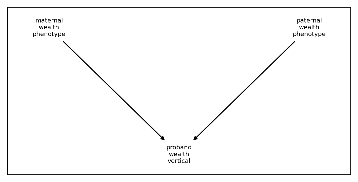
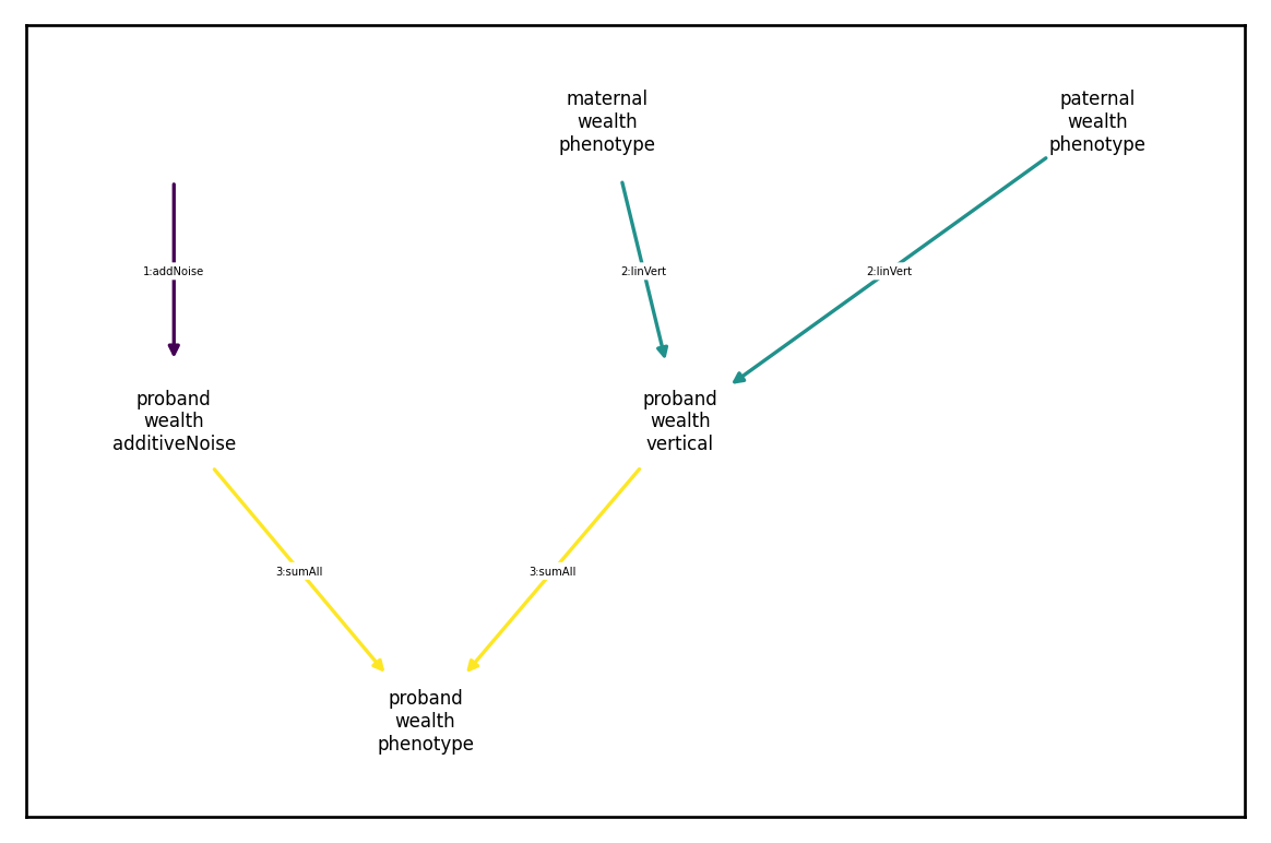
Vertical transmission
Univariate vertical transimission
Vertical transmission refers to causal dependence across parent and offspring generations. For example, we might want to model the inheritance of wealth across generations. One generative generative model could look like this:
I.e., half of wealth is individual specific noise and half is inherited from ones parents.
Specifying a linear transmission like this is quite similar to the previous example of causal dependencies, only the inputs refer to parent generation (as specified by vorigin_relative; see the tutorial on component indexing for further details) rather than the offspring generation. However, in addition to specifying the transmission as a linear opeartion, we have to specify a way to initialize the transmitted component in the founder generation. By default, we set
to this to independent Gaussian noise with user-supplied variance \(\sigma^2_\text{founder}\) such that \(\text{Wealth}_\text{vertical}\) is drawn from this distribution in the first generation (when, in the context of our simulation, no parents exist to pass on wealth).
We demonstrate this below:
[129]:
## noise component
ncomp = xft.arch.AdditiveNoiseComponent(variances=[.5],
                                        phenotype_name=['wealth'])

## transmitted component:
vert_input = xft.index.ComponentIndex.from_product(['wealth'], ['phenotype'], [0,1])
vert_input.comp_type ='output'
vert_output = xft.index.ComponentIndex.from_product(['wealth'], ['vertical'], [-1])
founder_variances = np.sqrt([.5,.5]) ## must be same length is inputs
coefficient_matrix = np.array([[np.sqrt(.25),np.sqrt(.25)]])

vtcomp = xft.arch.LinearVerticalComponent(input_cindex=vert_input,
                                          output_cindex=vert_output,
                                          founder_variances=founder_variances,
                                          coefficient_matrix=coefficient_matrix,
                                          normalize = False)
plt.rcParams['figure.figsize'] = [6.,3.]
vtcomp.draw_dependency_graph()
vtcomp
[129]:
<LinearVerticalComponent>
                                 wealth phenotype 0 output  \
wealth_vertical_-1_intermediate                        0.5

                                 wealth phenotype 1 output
wealth_vertical_-1_intermediate                        0.5
[130]:
plt.rcParams['figure.figsize'] = [6.,4.]

sind = xft.index.ComponentIndex.from_product(['wealth'],
                                             ['additiveNoise','vertical'])

strans = xft.arch.SumAllTransformation(input_cindex=sind)

test_sim = xft.sim.Simulation(founder_haplotypes=demo.haplotypes,
                              mating_regime=demo.mating_regime,
                              recombination_map= demo.recombination_map,
                              architecture = xft.arch.Architecture([ncomp, vtcomp, strans]),
                              statistics=[xft.stats.SampleStatistics()],)
test_sim.architecture.draw_dependency_graph()
test_sim.run(2)
pd = test_sim.phenotypes.xft.as_pd()
pd.corr()**2
[130]:
| phenotype_name | wealth | ||||||
|---|---|---|---|---|---|---|---|
| component_name | additiveNoise | phenotype | vertical | phenotype | |||
| vorigin_relative | proband | mother | father | proband | proband | ||
| phenotype_name | component_name | vorigin_relative | |||||
| wealth | additiveNoise | proband | 1.000000 | 0.000080 | 0.000005 | 0.000022 | 0.538641 |
| phenotype | mother | 0.000080 | 1.000000 | 0.000036 | 0.482565 | 0.228866 | |
| father | 0.000005 | 0.000036 | 1.000000 | 0.511408 | 0.234387 | ||
| vertical | proband | 0.000022 | 0.482565 | 0.511408 | 1.000000 | 0.466029 | |
| phenotype | proband | 0.538641 | 0.228866 | 0.234387 | 0.466029 | 1.000000 | |
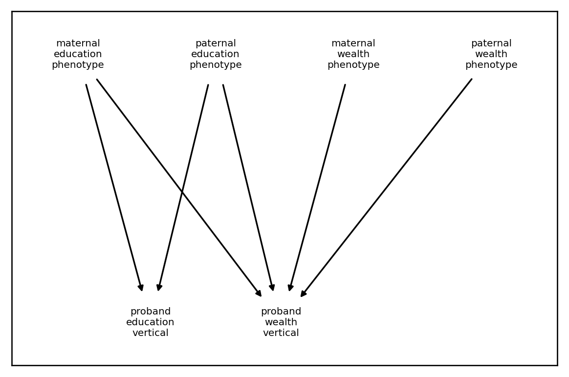
Multivariate vertical transimission
We might have more complex patterns of inheritance. For example, consider the following generative model:
where
at generation zero and
every subsequent generation, where \(\tilde{[\cdot]}\) denotes a standardized quantity. Under this model, half the variance in wealth and education are both independent Gaussian noise, half the variance in education is attributable to parental education, and a quarter each of the variance in wealth is attributable to parental education and parental wealth, respectively. We code this as follows:
[132]:
## noise component
ncomp = xft.arch.AdditiveNoiseComponent(variances=[.5,.5],
                                        phenotype_name=['education', 'wealth'])

## transmitted component:
vert_input = xft.index.ComponentIndex.from_product(['education', 'wealth'], ['phenotype'], [0,1])
vert_input.comp_type ='output'
vert_output = xft.index.ComponentIndex.from_product(['education', 'wealth'], ['vertical'], [-1])
founder_variances = np.sqrt([.5,.5,.5,.5]) ## must be same length is inputs
coefficient_matrix = np.array([[np.sqrt(.25),np.sqrt(.125)],
                               [np.sqrt(.25),np.sqrt(.125)],
                               [np.sqrt(0),np.sqrt(.125)],
                               [np.sqrt(0),np.sqrt(.125)],
                              ]).T

vtcomp = xft.arch.LinearVerticalComponent(input_cindex=vert_input,
                                          output_cindex=vert_output,
                                          founder_variances=founder_variances,
                                          coefficient_matrix=coefficient_matrix,
                                          normalize = True)
vtcomp.draw_dependency_graph()
vtcomp
[132]:
<LinearVerticalComponent>
                                    normalized_education phenotype 0 output  \
education_vertical_-1_intermediate                                 0.500000
wealth_vertical_-1_intermediate                                    0.353553

                                    normalized_education phenotype 1 output  \
education_vertical_-1_intermediate                                 0.500000
wealth_vertical_-1_intermediate                                    0.353553

                                    normalized_wealth phenotype 0 output  \
education_vertical_-1_intermediate                              0.000000
wealth_vertical_-1_intermediate                                 0.353553

                                    normalized_wealth phenotype 1 output
education_vertical_-1_intermediate                              0.000000
wealth_vertical_-1_intermediate                                 0.353553
[133]:
sind = xft.index.ComponentIndex.from_product(['education','wealth'],
                                             ['additiveNoise','vertical'])

strans = xft.arch.SumAllTransformation(input_cindex=sind)

test_sim = xft.sim.Simulation(founder_haplotypes=demo.haplotypes,
                              mating_regime=demo.mating_regime,
                              recombination_map= demo.recombination_map,
                              architecture = xft.arch.Architecture([ncomp, vtcomp, strans]),
                              statistics=[xft.stats.SampleStatistics()],)

test_sim.run(1)
pd = test_sim.phenotypes.xft.as_pd()
pd.corr()**2
[133]:
| phenotype_name | education | wealth | education | wealth | education | wealth | education | wealth | ||||
|---|---|---|---|---|---|---|---|---|---|---|---|---|
| component_name | additiveNoise | additiveNoise | phenotype | phenotype | vertical | vertical | phenotype | phenotype | ||||
| vorigin_relative | proband | proband | mother | father | mother | father | proband | proband | proband | proband | ||
| phenotype_name | component_name | vorigin_relative | ||||||||||
| education | additiveNoise | proband | 1.000000 | 0.000250 | 0.000503 | 0.000004 | 0.000298 | 0.001194 | 0.000303 | 0.000013 | 0.498270 | 0.000184 |
| wealth | additiveNoise | proband | 0.000250 | 1.000000 | 0.001502 | 0.000236 | 0.000244 | 0.000886 | 0.001486 | 0.000394 | 0.000254 | 0.510681 |
| education | phenotype | mother | 0.000503 | 0.001502 | 1.000000 | 0.000209 | 0.000741 | 0.000832 | 0.492767 | 0.267718 | 0.231546 | 0.151452 |
| father | 0.000004 | 0.000236 | 0.000209 | 1.000000 | 0.000260 | 0.000356 | 0.492767 | 0.241013 | 0.245884 | 0.125486 | ||
| wealth | phenotype | mother | 0.000298 | 0.000244 | 0.000741 | 0.000260 | 1.000000 | 0.000328 | 0.000063 | 0.243324 | 0.000046 | 0.126788 |
| father | 0.001194 | 0.000886 | 0.000832 | 0.000356 | 0.000328 | 1.000000 | 0.001154 | 0.261587 | 0.002390 | 0.113560 | ||
| education | vertical | proband | 0.000303 | 0.001486 | 0.492767 | 0.492767 | 0.000063 | 0.001154 | 1.000000 | 0.515842 | 0.484328 | 0.280384 |
| wealth | vertical | proband | 0.000013 | 0.000394 | 0.267718 | 0.241013 | 0.243324 | 0.261587 | 0.515842 | 1.000000 | 0.256310 | 0.509178 |
| education | phenotype | proband | 0.498270 | 0.000254 | 0.231546 | 0.245884 | 0.000046 | 0.002390 | 0.484328 | 0.256310 | 1.000000 | 0.133510 |
| wealth | phenotype | proband | 0.000184 | 0.510681 | 0.151452 | 0.125486 | 0.126788 | 0.113560 | 0.280384 | 0.509178 | 0.133510 | 1.000000 |
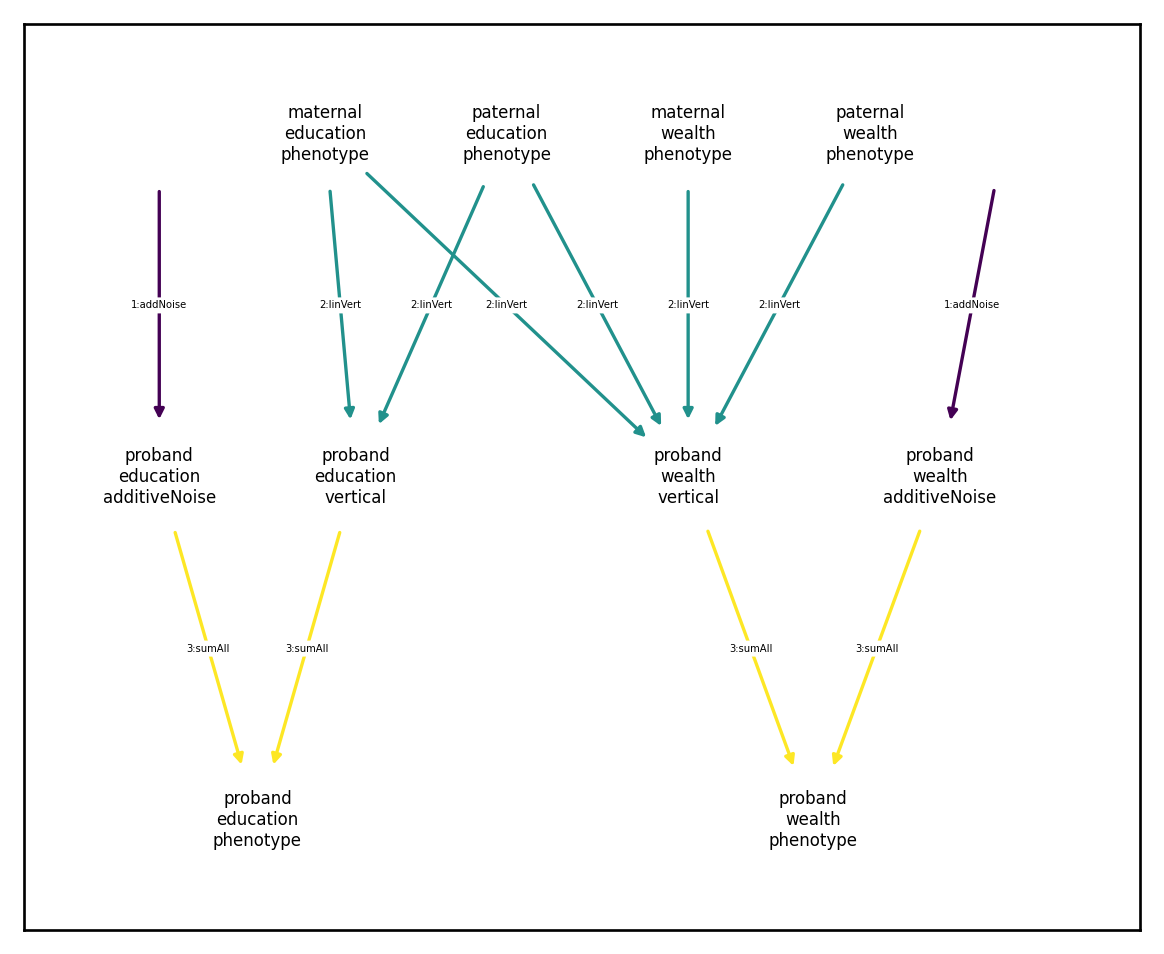
[134]:
plt.rcParams['figure.figsize'] = [6.,5.] ## better looking plots
xft.arch.Architecture([ncomp, vtcomp, strans]).draw_dependency_graph()
Product components
It’s common to model component interactions (as in gene-by-environment [GxE] interactions). In xftsim we can specify a ProductComponent, which requires the following:
input_cindex: the component index of the inputs to multiply togetheroutput_cindex: the component index of the output componentoutput_coef: optional coefficient to multiply product bycoefficient_vector: optional coefficents to multiply individual inputs by (usually only useful if three or more inputs are involvedmean_deviate: whether or not to mean-deviate inputs prior to multiplication, defaults toTruenormalize: whether or not to mean-deviate and standardize inputs prior to multiplication, defaults toFalse
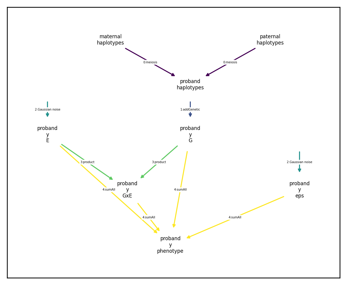
GxE interactions
The most common GxE model is a variant of the following:
We can model \(G\), \(E\), and \(\varepsilon\) using the already introduced noise and additive genetic components:
[135]:
## parameters
vg=.3
ve=.3
veps=.3
vgxe=.1
alpha=np.sqrt(vgxe/(vg*ve))


## architecture components
g_comp = xft.arch.AdditiveGeneticComponent(
    xft.effect.GCTAEffects(vg = [vg],
                           variant_indexer=demo.haplotypes.xft.get_variant_indexer(),
                           component_indexer=xft.index.ComponentIndex.from_product('y', 'G'))
)
e_eps_comp = xft.arch.AdditiveNoiseComponent(variances=[ve, veps],
                                             component_index=xft.index.ComponentIndex.from_product('y', ['E','eps']),
                                             component_name='Gaussian noise')
We then can add the GxE component using ProductComponent, then sum them all using a SumAllTransformation
[136]:
gxe_comp = xft.arch.ProductComponent(input_cindex=xft.index.ComponentIndex.from_product('y', ['G','E']),
                                     output_cindex=xft.index.ComponentIndex(['y'],['GxE']),
                                     output_coef=alpha,
                                     mean_deviate=False,
                                     normalize=False)

strans = xft.arch.SumAllTransformation(xft.index.ComponentIndex.from_product(['y'],
                                                                             ['G','E','eps','GxE']))
[137]:
gxe_arch = xft.arch.Architecture([g_comp,e_eps_comp,gxe_comp,strans])
demo = xft.sim.DemoSimulation()
gxe_sim = xft.sim.Simulation(founder_haplotypes=demo.haplotypes,
mating_regime=demo.mating_regime,
recombination_map= demo.recombination_map,
architecture = gxe_arch,
statistics=[xft.stats.SampleStatistics()],)
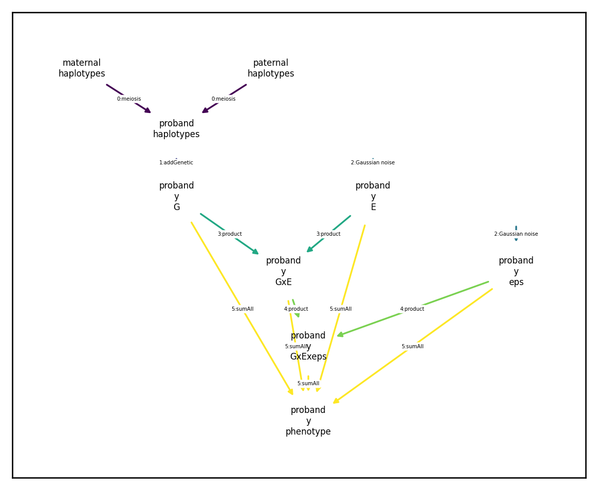
gxe_sim.run(1)
gxe_sim.draw_dependency_graph()
gxe_sim.results['sample_statistics']['variance_components']
[137]:
phenotype_name  component_name  vorigin_relative
y               G               proband             0.176002
                E               proband             0.171466
                eps             proband             0.175122
                GxE             proband             0.166555
dtype: float64
[138]:
np.hstack([gxe_sim.phenotypes.xft[{'component_name':'GxE'}].values,
           (gxe_sim.phenotypes.xft[{'component_name':'G'}].values * gxe_sim.phenotypes.xft[{'component_name':'E'}].values)])
[138]:
array([[-0.03146754, -0.02985273],
       [-0.15289007, -0.14504426],
       [-0.51998816, -0.49330408],
       ...,
       [-0.06002226, -0.05694212],
       [ 0.04044557,  0.03837004],
       [-0.15686073, -0.14881116]])
Higher-order interactions
To model higher order interactions, you simply need to specify multiple ProductComponents iteratively. For example, if for some reason we also wanted to include a \(G\times E\times\varepsilon\) interaction in the previous example, we could add a second ProductComponent as follows:
[139]:
gxexeps_comp = xft.arch.ProductComponent(input_cindex=xft.index.ComponentIndex.from_product('y', ['GxE','eps']),
                                     output_cindex=xft.index.ComponentIndex(['y'],['GxExeps']),
                                     output_coef=alpha,
                                     mean_deviate=True,
                                     normalize=False)

strans2 = xft.arch.SumAllTransformation(xft.index.ComponentIndex.from_product(['y'],
                                                                             ['G','E','eps','GxE','GxExeps']))
gxexeps_arch = xft.arch.Architecture([g_comp,e_eps_comp,gxe_comp,gxexeps_comp,strans2])
gxexeps_arch.draw_dependency_graph()
Sum transformations
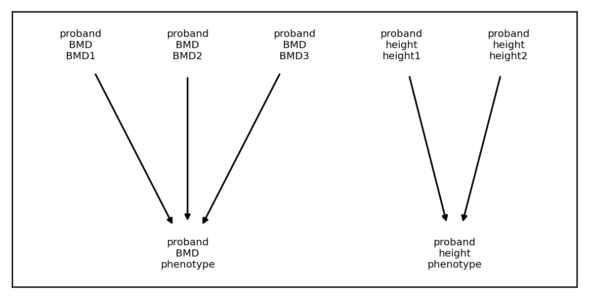
We nearly always will want to include a component that sums existing components to create composite phenotypes. This is straight forward to accomplish using the SumAllTransformation component. To specify a SumAllTransformation, we only need to provide the input component index and it will sum input components corresponding to the same phenotype:
[143]:
plt.rcParams['figure.figsize'] = [6.,3.]
input_cindex=xft.index.ComponentIndex(['BMD', 'BMD', 'BMD', 'height', 'height'],
                                      ['BMD1', 'BMD2', 'BMD3', 'height1', 'height2'])

strans = xft.arch.SumAllTransformation(input_cindex)
strans.draw_dependency_graph()
strans
[143]:
<class 'xftsim.arch.SumAllTransformation'>

## INPUTS:
 - haplotypes: False
 - phenotype components:
<ComponentIndex>
  5 components of 2 phenotypes spanning 1 generation
                       phenotype_name component_name  vorigin_relative  \
component
BMD.BMD1.proband                  BMD           BMD1                -1
BMD.BMD2.proband                  BMD           BMD2                -1
BMD.BMD3.proband                  BMD           BMD3                -1
height.height1.proband         height        height1                -1
height.height2.proband         height        height2                -1

                           comp_type
component
BMD.BMD1.proband        intermediate
BMD.BMD2.proband        intermediate
BMD.BMD3.proband        intermediate
height.height1.proband  intermediate
height.height2.proband  intermediate

## OUTPUTS:
 - phenotype components:
<ComponentIndex>
  1 component of 2 phenotypes spanning 1 generation
                         phenotype_name component_name  vorigin_relative  \
component
BMD.phenotype.proband               BMD      phenotype                -1
height.phenotype.proband         height      phenotype                -1

                         comp_type
component
BMD.phenotype.proband      outcome
height.phenotype.proband   outcome
Binarizations
Coming soon
Architecture objects: order matters
As we have seen throughout, an Architecture object is nothing more than a collection of ArchitectureComponents. These components are constructed in order (e.g., you can’t sum components that don’t yet exist), and can be arbitrarily complicated. We demonstrate a complex simulation below:

Here we assume that height is heritable with heritability 0.6, but that educational attainment and wealth are not. On the other hand, we assume that the variation in educational attainment is attributable in equal parts to parental educational attainment, parental wealth, and random noise. We also assume that an individual’s wealth is determined in equal parts by their own educational attainment, their parent’s wealth, and random noise. Thus we have additive genetic, additive noise, multivariate
vertical transmission, and causal dependence. We try to implement this in xftsim as follows:
[144]:
## This example won't work
founder_haplotypes = xft.founders.founder_haplotypes_uniform_AFs(n=4000,
                                                                 m=800)
rmap = xft.reproduce.RecombinationMap.constant_map_from_haplotypes(founder_haplotypes,
                                                                   .1)

genetic_effects = xft.effect.GCTAEffects(vg=[.6],
                                         variant_indexer=founder_haplotypes.xft.get_variant_indexer(),
                                         component_indexer=xft.index.ComponentIndex(['height'],
                                                                                    ['genetic']))
genetic_comp = xft.arch.AdditiveGeneticComponent(genetic_effects)

noise_comp = xft.arch.AdditiveNoiseComponent(variances=[.4,1/3,1/3],
                                             component_index=xft.index.ComponentIndex.from_product(['height','edu','wealth'],
                                                                                                   ['noise']))
vert_input = xft.index.ComponentIndex.from_product(['edu', 'wealth'], ['phenotype'], [0,1])
vert_input.comp_type ='output'
vert_output = xft.index.ComponentIndex.from_product(['edu', 'wealth'], ['vertical'], [-1])
founder_variances = np.sqrt([.5,.5,.5,.5]) ## must be same length is inputs
coefficient_matrix = np.array([[np.sqrt(1/3),np.sqrt(1/6)],
                               [np.sqrt(1/3),np.sqrt(1/6)],
                               [np.sqrt(0),np.sqrt(1/6)],
                               [np.sqrt(0),np.sqrt(1/6)],
                              ]).T

vt_comp = xft.arch.LinearVerticalComponent(input_cindex=vert_input,
                                          output_cindex=vert_output,
                                          founder_variances=[1.,1.,1.,1.,],
                                          coefficient_matrix=coefficient_matrix,
                                          normalize = True)
input_ind = xft.index.ComponentIndex(['edu'], ['phenotype'])
output_ind = xft.index.ComponentIndex(['wealth'], ['dependent'])
coefficient_matrix = np.array([[np.sqrt(1/3)]])

causal_comp = xft.arch.LinearTransformationComponent(input_ind, output_ind,
                                               coefficient_matrix, normalize = True)
input_cindex=xft.index.ComponentIndex(['height','height','edu', 'edu', 'wealth', 'wealth','wealth'],
                                      ['genetic','noise','noise', 'vertical', 'noise', 'vertical','dependent'])

strans = xft.arch.SumAllTransformation(input_cindex)

arch = xft.arch.Architecture([genetic_comp,
                              noise_comp,
                              causal_comp,
                              vt_comp,
                              strans])
/home/rsb/Dropbox/ftsim/xftsim/xftsim/arch.py:1620: UserWarning: Architecture contains out-of-order dependencies! This is probably a mistake, check dependency_graph using xft.arch.Architecture.draw_dependency_graph()
  warnings.warn('Architecture contains out-of-order dependencies! This is probably a mistake, check dependency_graph using xft.arch.Architecture.draw_dependency_graph()')
/home/rsb/Dropbox/ftsim/xftsim/xftsim/arch.py:1622: UserWarning: Architecture contains circular dependencies! This is probably a mistake, check dependency_graph using xft.arch.Architecture.draw_dependency_graph()
  warnings.warn('Architecture contains circular dependencies! This is probably a mistake, check dependency_graph using xft.arch.Architecture.draw_dependency_graph()')
[145]:
mating = xft.mate.LinearAssortativeMatingRegime(r=.25,
                                                component_index =xft.index.ComponentIndex.from_product(['edu', 'wealth','height'], ['phenotype']),
                                                offspring_per_pair=2,
                                                mates_per_female=1)
[146]:
sim = xft.sim.Simulation(architecture=arch,
                   founder_haplotypes=founder_haplotypes,
                   recombination_map=rmap,
                   mating_regime=mating,
                   statistics=[xft.stats.SampleStatistics(),
                               xft.stats.MatingStatistics(),
                               xft.stats.HasemanElstonEstimator(randomized=True)])
sim.run(1)
sim.phenotypes.xft.as_pd()
[146]:
| phenotype_name | height | edu | wealth | edu | wealth | edu | wealth | edu | wealth | height | wealth | |||||
|---|---|---|---|---|---|---|---|---|---|---|---|---|---|---|---|---|
| component_name | genetic | noise | noise | noise | phenotype | dependent | phenotype | phenotype | vertical | vertical | phenotype | phenotype | ||||
| vorigin_relative | proband | proband | proband | proband | proband | proband | mother | father | mother | father | proband | proband | proband | proband | ||
| iid | fid | sex | ||||||||||||||
| 0_0 | 0_0 | 0 | 1.159406 | 0.227379 | 1.346853 | -1.009528 | 1.845065 | NaN | 0.703345 | 0.145432 | -0.715301 | 1.676621 | 0.498212 | 0.725893 | 1.386785 | NaN |
| 0_1 | 0_1 | 1 | 0.125946 | 0.253585 | 0.635969 | 0.324132 | 1.647804 | NaN | 2.025557 | -0.291935 | 0.209519 | -0.430877 | 1.011835 | 0.613009 | 0.379531 | NaN |
| 0_2 | 0_2 | 0 | 0.206073 | -0.167993 | -0.194083 | -0.042954 | 0.669267 | NaN | 1.453426 | 0.023931 | 0.637377 | -0.804260 | 0.863350 | 0.533613 | 0.038080 | NaN |
| 0_3 | 0_3 | 1 | -1.622558 | -0.993449 | 0.335210 | -0.659354 | 0.841432 | NaN | 0.668399 | 0.194043 | -0.898454 | -0.284408 | 0.506222 | -0.146064 | -2.616007 | NaN |
| 0_4 | 0_4 | 0 | 1.001216 | -0.203757 | -0.230779 | -0.650563 | -0.081440 | NaN | -1.502208 | 1.746790 | 0.444078 | -0.619185 | 0.149339 | 0.023862 | 0.797460 | NaN |
| ... | ... | ... | ... | ... | ... | ... | ... | ... | ... | ... | ... | ... | ... | ... | ... | ... |
| 0_3995 | 0_3995 | 1 | 0.113787 | 0.234693 | -1.100652 | -0.745577 | -0.755603 | NaN | 1.329808 | -0.742415 | 2.716830 | -2.112150 | 0.345049 | 0.498633 | 0.348480 | NaN |
| 0_3996 | 0_3996 | 0 | 1.160719 | -1.175063 | 0.260536 | 0.566314 | -0.390905 | NaN | 0.694559 | -1.819184 | 0.441658 | 0.820460 | -0.651441 | 0.044909 | -0.014344 | NaN |
| 0_3997 | 0_3997 | 1 | -0.246167 | -0.648348 | -0.295313 | -0.068992 | 0.422221 | NaN | 1.478913 | -0.251788 | -0.036908 | -1.560748 | 0.717533 | -0.159423 | -0.894514 | NaN |
| 0_3998 | 0_3998 | 0 | -0.694219 | -0.696193 | -0.018587 | -0.612840 | -0.296463 | NaN | -0.474250 | -0.011987 | -0.383620 | -0.903747 | -0.277876 | -0.739193 | -1.390411 | NaN |
| 0_3999 | 0_3999 | 1 | -0.891533 | 0.768979 | 0.011346 | -0.578812 | 0.260793 | NaN | 1.319061 | -0.895793 | 0.213371 | -0.606629 | 0.249448 | 0.003705 | -0.122554 | NaN |
4000 rows × 14 columns
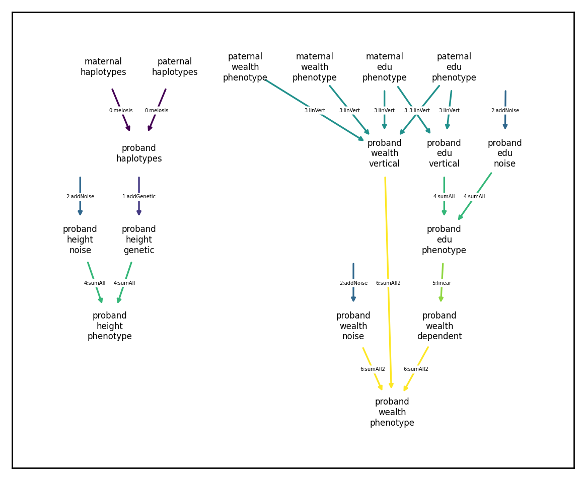
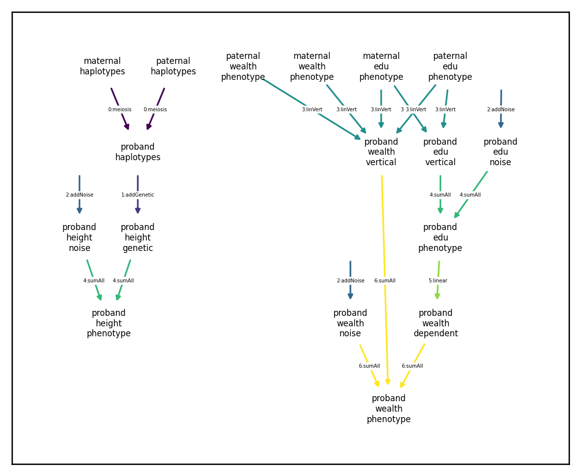
It looks like the simulation wasn’t able to compute the ‘dependent’ or ‘phenotype’ components of ‘wealth’. What happened here? Looking at the dependency graph (which colors edges in order of computation) we see we have a circular dependency:
[147]:
plt.rcParams['figure.figsize'] = [6.,5.]
arch.draw_dependency_graph(font_size=5, node_size=1000)
Specifically, the edu phenotype node generated by the sum transformation (yellow arrows) but has a causal effect (teal arrow) on the wealth dependent component, which is again used by the sum transformation to construct the wealth phenotype component.
Avoiding circular dependences
There are multiple ways to avoid this sort of circular dependency. The first would be to have the wealth dependent component depend directly on edu noise and edu vertical:
[148]:
input_ind = xft.index.ComponentIndex.from_product(['edu'], ['noise', 'vertical'])
output_ind = xft.index.ComponentIndex(['wealth'], ['dependent'])
coefficient_matrix = np.array([[np.sqrt(1/6),np.sqrt(1/6)]])

causal_comp_redux = xft.arch.LinearTransformationComponent(input_ind, output_ind,
                                               coefficient_matrix, normalize = True)
input_cindex=xft.index.ComponentIndex(['height','height','edu', 'edu', 'wealth', 'wealth','wealth'],
                                      ['genetic','noise','noise', 'vertical', 'noise', 'vertical','dependent'])

strans = xft.arch.SumAllTransformation(input_cindex)

arch_redux1 = xft.arch.Architecture([genetic_comp,
                                     noise_comp,
                                     vt_comp,
                                     causal_comp_redux,
                                     strans])
arch_redux1.draw_dependency_graph(font_size=5, node_size=1000)
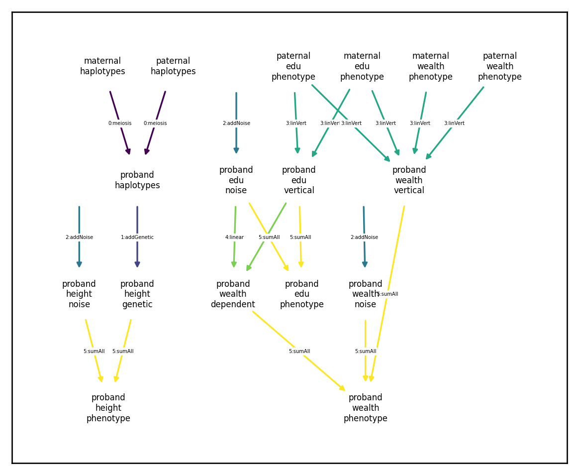
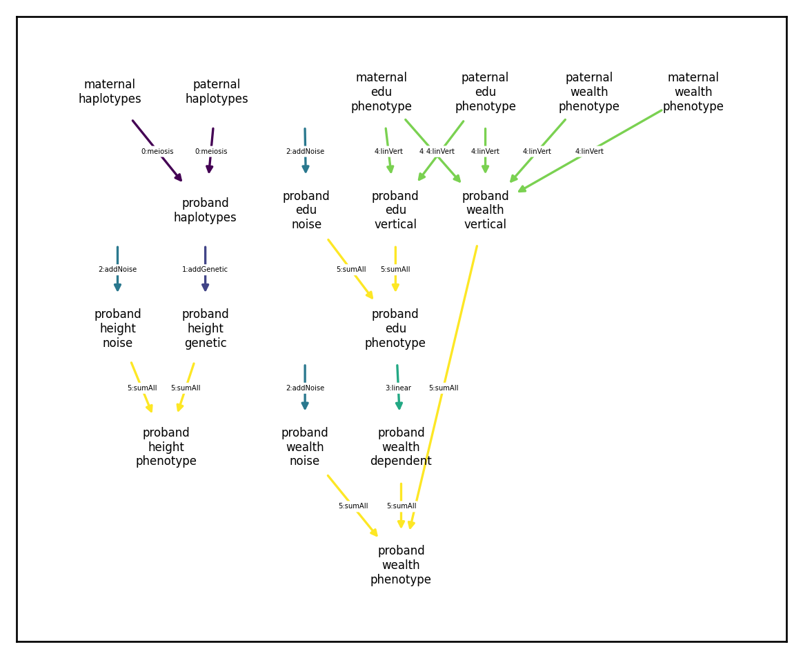
We can tell that there are no circular dependencies because all directed paths through the network travel through each color at most once. An alternative method for avoid circular dependences would be to keep the dependence between wealth dependent and edu phenotype but compute the sums in two steps:
[149]:
input_cindex=xft.index.ComponentIndex(['height','height','edu', 'edu'],
                                      ['genetic','noise','noise', 'vertical'])

strans_redux1 = xft.arch.SumAllTransformation(input_cindex)

input_cindex=xft.index.ComponentIndex(['wealth', 'wealth','wealth'],
                                      ['noise', 'vertical','dependent'])

strans_redux2 = xft.arch.SumAllTransformation(input_cindex)


arch_redux2 = xft.arch.Architecture([genetic_comp,
                                     noise_comp,
                                     vt_comp,
                                     strans_redux1,
                                     causal_comp,
                                     strans_redux2])
arch_redux2.draw_dependency_graph(font_size=5, node_size=800)
Both of these reformulations are equivalent and will produce expected results:
[150]:
sim_redux1 = xft.sim.Simulation(architecture=arch_redux1,
                   founder_haplotypes=founder_haplotypes,
                   recombination_map=rmap,
                   mating_regime=mating,
                   statistics=[xft.stats.SampleStatistics(),
                               xft.stats.MatingStatistics(),
                               xft.stats.HasemanElstonEstimator(randomized=True)])
sim_redux1.run(1)
sim_redux1.phenotypes.xft.as_pd()
[150]:
| phenotype_name | height | edu | wealth | edu | wealth | edu | wealth | height | edu | wealth | ||||||
|---|---|---|---|---|---|---|---|---|---|---|---|---|---|---|---|---|
| component_name | genetic | noise | noise | noise | phenotype | phenotype | vertical | vertical | dependent | phenotype | phenotype | phenotype | ||||
| vorigin_relative | proband | proband | proband | proband | mother | father | mother | father | proband | proband | proband | proband | proband | proband | ||
| iid | fid | sex | ||||||||||||||
| 0_0 | 0_0 | 0 | 1.159406 | -0.117105 | 0.220000 | 0.915644 | -0.739280 | -0.807028 | 0.212879 | 1.561457 | -0.914153 | 0.096066 | -0.305832 | 1.042301 | -0.694153 | 0.705877 |
| 0_1 | 0_1 | 1 | 0.125946 | -0.266341 | 0.195536 | 0.985539 | -2.239504 | 1.248151 | 2.148847 | -0.025985 | -0.593081 | 0.451099 | -0.161042 | -0.140395 | -0.397545 | 1.275596 |
| 0_2 | 0_2 | 0 | 0.206073 | -0.567942 | -0.348266 | 0.583431 | 0.016963 | 0.871919 | -0.547299 | -0.537265 | 0.510291 | -0.074955 | 0.008194 | -0.361870 | 0.162026 | 0.516670 |
| 0_3 | 0_3 | 1 | -1.622558 | 0.291262 | -0.344397 | 1.026636 | -0.190218 | -0.696956 | -0.483706 | -1.295044 | -0.527868 | -1.097249 | -0.513706 | -1.331295 | -0.872264 | -0.584319 |
| 0_4 | 0_4 | 0 | 1.001216 | 0.839900 | -0.083416 | -0.419417 | 0.149244 | 0.899875 | -0.421356 | 0.319231 | 0.604195 | 0.397491 | 0.244808 | 1.841117 | 0.520779 | 0.222882 |
| ... | ... | ... | ... | ... | ... | ... | ... | ... | ... | ... | ... | ... | ... | ... | ... | ... |
| 0_3995 | 0_3995 | 1 | 0.113787 | -1.691715 | 0.345358 | -0.292176 | -0.347452 | 0.568217 | -0.583026 | 1.530001 | 0.119149 | 0.490622 | 0.305908 | -1.577927 | 0.464508 | 0.504354 |
| 0_3996 | 0_3996 | 0 | 1.160719 | -0.399978 | 1.036688 | 0.672909 | 0.982978 | -1.995735 | 1.499277 | -0.377633 | -0.598758 | 0.037699 | 0.436843 | 0.760742 | 0.437930 | 1.147451 |
| 0_3997 | 0_3997 | 1 | -0.246167 | -0.565388 | -0.261406 | 0.112722 | 2.299636 | 0.800685 | 0.137146 | -0.189149 | 1.807237 | 1.264202 | 0.725678 | -0.811555 | 1.545830 | 2.102602 |
| 0_3998 | 0_3998 | 0 | -0.694219 | -1.238411 | 0.180182 | 0.182042 | -2.019804 | -2.063854 | -0.262075 | 1.267582 | -2.399399 | -1.268728 | -1.084882 | -1.932629 | -2.219217 | -2.171568 |
| 0_3999 | 0_3999 | 1 | -0.891533 | -0.373617 | 0.602778 | 0.262371 | 0.282297 | -0.940999 | 0.024815 | -1.904895 | -0.393374 | -1.048453 | 0.230740 | -1.265150 | 0.209404 | -0.555342 |
4000 rows × 14 columns
[151]:
sim_redux2 = xft.sim.Simulation(architecture=arch_redux2,
                   founder_haplotypes=founder_haplotypes,
                   recombination_map=rmap,
                   mating_regime=mating,
                   statistics=[xft.stats.SampleStatistics(),
                               xft.stats.MatingStatistics(),
                               xft.stats.HasemanElstonEstimator(randomized=True)])
sim_redux2.run(1)
sim_redux2.phenotypes.xft.as_pd()
[151]:
| phenotype_name | height | edu | wealth | edu | wealth | edu | wealth | height | edu | wealth | ||||||
|---|---|---|---|---|---|---|---|---|---|---|---|---|---|---|---|---|
| component_name | genetic | noise | noise | noise | phenotype | phenotype | vertical | vertical | phenotype | phenotype | dependent | phenotype | ||||
| vorigin_relative | proband | proband | proband | proband | mother | father | mother | father | proband | proband | proband | proband | proband | proband | ||
| iid | fid | sex | ||||||||||||||
| 0_0 | 0_0 | 0 | 1.159406 | -0.546539 | -1.001797 | 0.349617 | -1.108498 | -0.324742 | -0.177253 | -0.298432 | -0.842509 | -0.792662 | 0.612867 | -1.844306 | -1.084443 | -1.527489 |
| 0_1 | 0_1 | 1 | 0.125946 | 0.211568 | 0.655474 | -0.658234 | -0.014737 | 0.649331 | 0.023321 | -1.044911 | 0.364343 | -0.168779 | 0.337514 | 1.019817 | 0.586801 | -0.240213 |
| 0_2 | 0_2 | 0 | 0.206073 | 0.449290 | -0.617535 | 0.361389 | 0.345194 | 0.652465 | -1.958641 | -0.795011 | 0.575796 | -0.726939 | 0.655363 | -0.041739 | -0.032628 | -0.398177 |
| 0_3 | 0_3 | 1 | -1.622558 | 0.605143 | 0.421832 | -0.082621 | -1.475429 | -0.869364 | 0.255666 | -0.380774 | -1.374825 | -1.026077 | -1.017415 | -0.952992 | -0.564353 | -1.673051 |
| 0_4 | 0_4 | 0 | 1.001216 | -0.292512 | -0.749755 | 1.021507 | 0.570206 | 0.832566 | -1.317082 | -0.730567 | 0.812205 | -0.270018 | 0.708704 | 0.062450 | 0.028167 | 0.779656 |
| ... | ... | ... | ... | ... | ... | ... | ... | ... | ... | ... | ... | ... | ... | ... | ... | ... |
| 0_3995 | 0_3995 | 1 | 0.113787 | -0.511680 | -0.325261 | -0.068777 | 0.296796 | 0.047564 | -0.471232 | 1.269533 | 0.193727 | 0.474273 | -0.397892 | -0.131534 | -0.085024 | 0.320472 |
| 0_3996 | 0_3996 | 0 | 1.160719 | -0.000059 | -0.686439 | -0.093433 | -0.535602 | -0.107938 | -0.223625 | -0.321829 | -0.382025 | -0.495818 | 1.160661 | -1.068464 | -0.631732 | -1.220983 |
| 0_3997 | 0_3997 | 1 | -0.246167 | -0.818587 | 0.859880 | -0.481383 | -0.440180 | 0.153001 | -0.265414 | 1.154747 | -0.173796 | 0.250794 | -1.064754 | 0.686084 | 0.392064 | 0.161475 |
| 0_3998 | 0_3998 | 0 | -0.694219 | 0.894682 | 0.558028 | 0.672593 | 0.254668 | 0.783876 | 0.294473 | -0.350325 | 0.599954 | 0.398915 | 0.200463 | 1.157982 | 0.667421 | 1.738929 |
| 0_3999 | 0_3999 | 1 | -0.891533 | -0.471611 | -1.152219 | 0.209416 | -0.299089 | 0.808012 | -0.094723 | -0.409097 | 0.291572 | -0.003137 | -1.363144 | -0.860646 | -0.510468 | -0.304190 |
4000 rows × 14 columns
We can give each a custom name for displaying on the dependency graph using the component_name argument.
[152]:
input_cindex=xft.index.ComponentIndex(['wealth', 'wealth','wealth'],
                                      ['noise', 'vertical','dependent'])

strans_redux3 = xft.arch.SumAllTransformation(input_cindex,
                                              component_name='sumAll2')


arch_redux3 = xft.arch.Architecture([genetic_comp,
                                     noise_comp,
                                     vt_comp,
                                     strans_redux1,
                                     causal_comp,
                                     strans_redux3])
arch_redux3.draw_dependency_graph(font_size=5, node_size=800, arrowsize=5)